1 Goals for Lab 05

Goal: Become familiar with tools for generating publication-ready tables directly in R.

We will use data from the following paper: MacFarlane, H., Gorman, K., Ingham, R., Presmanes Hill, A., Papadakis, K., Kiss, G., & van Santen, J. (2017). Quantitative analysis of disfluency in children with autism spectrum disorder or language impairment. PLoS ONE, 12(3), e0173936.

mazes <- read_csv("data/mazes.csv") %>% 
  clean_names()  #janitor package

glimpse(mazes)

Rows: 381
Columns: 12
$ study_id <chr> "CSLU-001", "CSLU-001", "CSLU-001", "CSLU-001", "CSLU-002", "CSLU-002", "CSLU-002", "CSLU-002", "CSLU-007", "CSLU-007", "C…
$ ca       <dbl> 5.6667, 5.6667, 5.6667, 5.6667, 6.5000, 6.5000, 6.5000, 6.5000, 7.5000, 7.5000, 7.5000, 7.5000, 5.2500, 5.2500, 5.2500, 5.…
$ viq      <dbl> 124, 124, 124, 124, 124, 124, 124, 124, 108, 108, 108, 108, 112, 112, 112, 112, 102, 102, 102, 102, 102, 102, 102, 102, 81…
$ dx       <chr> "TD", "TD", "TD", "TD", "TD", "TD", "TD", "TD", "TD", "TD", "TD", "TD", "TD", "TD", "TD", "TD", "ASD", "ASD", "ASD", "ASD"…
$ activity <chr> "Conversation", "Picture Description", "Play", "Wordless Picture Book", "Conversation", "Picture Description", "Play", "Wo…
$ content  <dbl> 24, 1, 21, 8, 3, 5, 8, 2, 25, 10, 2, 5, 32, 20, 13, 21, 27, 9, 12, 6, 60, 36, 17, 14, 30, 21, 54, 17, 27, 4, 10, 8, 7, 8, …
$ filler   <dbl> 31, 2, 6, 2, 10, 3, 8, 2, 21, 13, 10, 2, 12, 9, 4, 4, 12, 6, 7, 3, 23, 6, 4, 6, 6, 2, 5, 0, 18, 5, 9, 0, 1, 2, 2, 17, 5, 2…
$ rep      <dbl> 2, 0, 3, 0, 3, 2, 3, 0, 4, 0, 0, 0, 13, 5, 5, 6, 10, 5, 5, 2, 20, 16, 3, 3, 17, 8, 26, 6, 4, 1, 1, 2, 5, 5, 3, 8, 4, 4, 4,…
$ rev      <dbl> 5, 0, 8, 4, 0, 1, 2, 0, 4, 2, 1, 3, 8, 7, 2, 8, 5, 1, 4, 2, 19, 10, 7, 2, 4, 2, 11, 5, 7, 2, 5, 2, 1, 0, 1, 10, 1, 5, 4, 1…
$ fs       <dbl> 17, 1, 10, 4, 0, 2, 3, 2, 17, 8, 1, 2, 11, 8, 6, 7, 12, 3, 3, 2, 21, 10, 7, 9, 9, 11, 17, 6, 16, 1, 4, 4, 1, 3, 0, 18, 9, …
$ cued     <dbl> 36, 2, 6, 2, 10, 3, 9, 2, 29, 13, 11, 2, 14, 12, 4, 11, 17, 7, 9, 4, 27, 11, 5, 10, 7, 2, 7, 0, 24, 5, 12, 0, 1, 2, 3, 29,…
$ not_cued <dbl> 50, 3, 27, 10, 13, 8, 15, 4, 38, 23, 11, 7, 42, 26, 17, 18, 34, 14, 17, 8, 79, 37, 20, 16, 35, 23, 57, 17, 39, 9, 16, 8, 8…

2 TL;DR

The workhorse for making simple tables in R Markdown documents is the knitr package’s kable function. This function is really versatile, but also free of fancy formatting options, for better or worse.

3 `knitr::kable`

3.1 `kable` all tables everywhere

In order to tell RMarkdown to use kable to format all tabular output, update the YAML header in your document and override the df_print option, when producing HTML output:

---
title: "My Awesome Data Vis Lab"
output:
  html_document:
    df_print: kable
---

You can also define the html format in the global options.

# If you don't define format here, you'll need put `format = "html"` in every kable function.
options(knitr.table.format = "html") 
# You may also wish to set this option, to handle number formatting
options(scipen = 1, digits = 2)

3.2 `kable` table in a chunk

For HTML output:

head(mazes) %>% 
  kable(format = "html")

study_id	ca	viq	dx	activity	content	filler	rep	rev	fs	cued	not_cued
CSLU-001	5.6667	124	TD	Conversation	24	31	2	5	17	36	50
CSLU-001	5.6667	124	TD	Picture Description	1	2	0	0	1	2	3
CSLU-001	5.6667	124	TD	Play	21	6	3	8	10	6	27
CSLU-001	5.6667	124	TD	Wordless Picture Book	8	2	0	4	4	2	10
CSLU-002	6.5000	124	TD	Conversation	3	10	3	0	0	10	13
CSLU-002	6.5000	124	TD	Picture Description	5	3	2	1	2	3	8

Note that this is a bit rough-looking. We will use various features of kable to improve our output.

For starters, we can add a caption:

head(mazes) %>% 
  kable(format = "html", digits = 2, caption = "A table produced by kable.")

A table produced by kable.
study_id	ca	viq	dx	activity	content	filler	rep	rev	fs	cued	not_cued
CSLU-001	5.67	124	TD	Conversation	24	31	2	5	17	36	50
CSLU-001	5.67	124	TD	Picture Description	1	2	0	0	1	2	3
CSLU-001	5.67	124	TD	Play	21	6	3	8	10	6	27
CSLU-001	5.67	124	TD	Wordless Picture Book	8	2	0	4	4	2	10
CSLU-002	6.50	124	TD	Conversation	3	10	3	0	0	10	13
CSLU-002	6.50	124	TD	Picture Description	5	3	2	1	2	3	8

We can also manually specify human-readable column names:

my_maze_names <- c("Participant", "Age", "Verbal\nIQ", "Group", "Activity", "Content\nMaze", "Filler\nMaze", "Repetition", "Revision", "False\nStart", "Cued", "Not\nCued")
head(mazes) %>% 
  kable(format = "html", digits = 2, caption = "A table produced by kable.",
        col.names = my_maze_names)

A table produced by kable.
Participant	Age	Verbal IQ	Group	Activity	Content Maze	Filler Maze	Repetition	Revision	False Start	Cued	Not Cued
CSLU-001	5.67	124	TD	Conversation	24	31	2	5	17	36	50
CSLU-001	5.67	124	TD	Picture Description	1	2	0	0	1	2	3
CSLU-001	5.67	124	TD	Play	21	6	3	8	10	6	27
CSLU-001	5.67	124	TD	Wordless Picture Book	8	2	0	4	4	2	10
CSLU-002	6.50	124	TD	Conversation	3	10	3	0	0	10	13
CSLU-002	6.50	124	TD	Picture Description	5	3	2	1	2	3	8

3.3 Styled `kable` tables in a chunk

To improve the visual layout of the table, we can use the kableExtra package, which provides the kable_styling() function:

head(mazes) %>% 
  kable(format = "html", digits = 2, caption = "A styled kable table.",
        col.names = my_maze_names) %>% 
  kable_styling()

A styled kable table.
Participant	Age	Verbal IQ	Group	Activity	Content Maze	Filler Maze	Repetition	Revision	False Start	Cued	Not Cued
CSLU-001	5.67	124	TD	Conversation	24	31	2	5	17	36	50
CSLU-001	5.67	124	TD	Picture Description	1	2	0	0	1	2	3
CSLU-001	5.67	124	TD	Play	21	6	3	8	10	6	27
CSLU-001	5.67	124	TD	Wordless Picture Book	8	2	0	4	4	2	10
CSLU-002	6.50	124	TD	Conversation	3	10	3	0	0	10	13
CSLU-002	6.50	124	TD	Picture Description	5	3	2	1	2	3	8

There are lots of printing options: https://haozhu233.github.io/kableExtra/awesome_table_in_html.html

head(mazes) %>% 
  kable(format = "html", digits = 2, caption = "A non-full width zebra kable table.") %>% 
  kable_styling(bootstrap_options = "striped", full_width = F)

A non-full width zebra kable table.
study_id	ca	viq	dx	activity	content	filler	rep	rev	fs	cued	not_cued
CSLU-001	5.67	124	TD	Conversation	24	31	2	5	17	36	50
CSLU-001	5.67	124	TD	Picture Description	1	2	0	0	1	2	3
CSLU-001	5.67	124	TD	Play	21	6	3	8	10	6	27
CSLU-001	5.67	124	TD	Wordless Picture Book	8	2	0	4	4	2	10
CSLU-002	6.50	124	TD	Conversation	3	10	3	0	0	10	13
CSLU-002	6.50	124	TD	Picture Description	5	3	2	1	2	3	8

Note that by default the table will be centered; you can override this by specifying a position:

head(mazes) %>% 
  kable(format = "html", digits = 2, caption = "Over here!") %>% 
  kable_styling(bootstrap_options = "striped", full_width = F, position = "left")

Over here!
study_id	ca	viq	dx	activity	content	filler	rep	rev	fs	cued	not_cued
CSLU-001	5.67	124	TD	Conversation	24	31	2	5	17	36	50
CSLU-001	5.67	124	TD	Picture Description	1	2	0	0	1	2	3
CSLU-001	5.67	124	TD	Play	21	6	3	8	10	6	27
CSLU-001	5.67	124	TD	Wordless Picture Book	8	2	0	4	4	2	10
CSLU-002	6.50	124	TD	Conversation	3	10	3	0	0	10	13
CSLU-002	6.50	124	TD	Picture Description	5	3	2	1	2	3	8

3.4 Controlling column appearance

We can control the formatting of individual columns using the column_spec() function:

head(mazes) %>% 
  kable(format = "html", digits = 2, caption = "Over here!") %>% 
  kable_styling(bootstrap_options = "striped", full_width = F, position = "left") %>% 
  column_spec(4, width="3cm", background="lightblue", border_right=TRUE)

Over here!
study_id	ca	viq	dx	activity	content	filler	rep	rev	fs	cued	not_cued
CSLU-001	5.67	124	TD	Conversation	24	31	2	5	17	36	50
CSLU-001	5.67	124	TD	Picture Description	1	2	0	0	1	2	3
CSLU-001	5.67	124	TD	Play	21	6	3	8	10	6	27
CSLU-001	5.67	124	TD	Wordless Picture Book	8	2	0	4	4	2	10
CSLU-002	6.50	124	TD	Conversation	3	10	3	0	0	10	13
CSLU-002	6.50	124	TD	Picture Description	5	3	2	1	2	3	8

3.5 `kable` + `kableExtra` + `formattable`

color_tile and color_bar are neat extras, if used wisely and in moderation!

http://haozhu233.github.io/kableExtra/use_kableExtra_with_formattable.html

library(formattable)
head(mazes) %>% 
  mutate(ca = color_tile("transparent", "lightpink")(ca),
         viq = color_bar("lightseagreen")(viq)) %>%
  kable("html", escape = F, caption = 'This table is colored.') %>%
  kable_styling(position = "center") %>% 
  column_spec(4, width = "3cm")

This table is colored.
study_id	ca	viq	dx	activity	content	filler	rep	rev	fs	cued	not_cued
CSLU-001	5.6667	124	TD	Conversation	24	31	2	5	17	36	50
CSLU-001	5.6667	124	TD	Picture Description	1	2	0	0	1	2	3
CSLU-001	5.6667	124	TD	Play	21	6	3	8	10	6	27
CSLU-001	5.6667	124	TD	Wordless Picture Book	8	2	0	4	4	2	10
CSLU-002	6.5000	124	TD	Conversation	3	10	3	0	0	10	13
CSLU-002	6.5000	124	TD	Picture Description	5	3	2	1	2	3	8

3.6 `tibble` + `kable` + `kableExtra`

Sometimes, when writing a document or preparing a report, you may have tabular information to present that is not already in a dataframe. For example, consider the helpful table of vectorized math operators from one of the slide decks. I made this by first manually creating a data frame to hold the contents of the table (using the tibble package’s tribble() function), and then formatting it as before.

Manually creating a quick-and-dirty dataframe with tribble() is simple:

math_table <- tibble::tribble(
  ~Operator, ~Description, ~Usage, # column names
  "\\+", "addition", "x + y", # each column, for each row, separated by commas
  "\\-", "subtraction", "x - y",
  "\\*", "multiplication", "x * y",
  "/", "division", "x / y",
  "^", "raised to the power of", "x ^ y",
  "abs", "absolute value", "abs(x)",
  "%/%", "integer division", "x %/% y",
  "%%", "remainder after division", "x %% y"
)

Then I used this chunk to print it:

```{r, results = 'asis'}
knitr::kable(math_table, format = "html", caption = "Helpful mutate functions") %>% 
  kable_styling(bootstrap_options = "striped", full_width = F, position = "left")
```

knitr::kable(math_table, format = "html", caption = "Helpful mutate functions") %>% 
  kable_styling(bootstrap_options = "striped", full_width = F, position = "left")

Helpful mutate functions
Operator	Description	Usage
+	addition	x + y
-	subtraction	x - y
*	multiplication	x * y
/	division	x / y
^	raised to the power of	x ^ y
abs	absolute value	abs(x)
%/%	integer division	x %/% y
%%	remainder after division	x %% y

4 Markdown Tables

Alternatively, you may just want to type in a table in Markdown and ignore R. Four kinds of tables may be used. The first three kinds presuppose the use of a fixed-width (monospaced) font, such as Courier. The fourth method can be used with proportionally spaced fonts, as it does not require lining up columns. All of the below will render when typed outside of an R code chunk since these are based on pandoc being used to render your markdown document. Note that these should all work whether you are knitting to either html or PDF.

4.1 Simple table

This code for a simple table:

  Right     Left     Center     Default
-------     ------ ----------   -------
     12     12        12            12
    123     123       123          123
      1     1          1             1

Table:  Demonstration of simple table syntax.

Produces this simple table:

Demonstration of simple table syntax.
Right	Left	Center	Default
12	12	12	12
123	123	123	123
1	1	1	1

The headers and table rows must each fit on one line. Column alignments are determined by the position of the header text relative to the dashed line below it:3

If the dashed line is flush with the header text on the right side but extends beyond it on the left, the column is right-aligned.
If the dashed line is flush with the header text on the left side but extends beyond it on the right, the column is left-aligned.
If the dashed line extends beyond the header text on both sides, the column is centered.
If the dashed line is flush with the header text on both sides, the default alignment is used (in most cases, this will be left).
The table must end with a blank line, or a line of dashes followed by a blank line.

The column headers may be omitted, provided a dashed line is used to end the table.

4.2 Multi-line tables

This code for a multi-line table:

-------------------------------------------------------------
 Centered   Default           Right Left
  Header    Aligned         Aligned Aligned
----------- ------- --------------- -------------------------
   First    row                12.0 Example of a row that
                                    spans multiple lines.

  Second    row                 5.0 Here's another one. Note
                                    the blank line between
                                    rows.
-------------------------------------------------------------

Table: Here's the caption. It, too, may span
multiple lines.

Produces this multi-line table:

Here’s the caption. It, too, may span multiple lines.
Centered Header	Default Aligned	Right Aligned	Left Aligned
First	row	12.0	Example of a row that spans multiple lines.
Second	row	5.0	Here’s another one. Note the blank line between rows.

4.3 Grid tables

This code for a grid table:

: Sample grid table.

+---------------+---------------+--------------------+
| Fruit         | Price         | Advantages         |
+===============+===============+====================+
| Bananas       | $1.34         | - built-in wrapper |
|               |               | - bright color     |
+---------------+---------------+--------------------+
| Oranges       | $2.10         | - cures scurvy     |
|               |               | - tasty            |
+---------------+---------------+--------------------+

Produces this grid table:

Sample grid table.
Fruit	Price	Advantages
Bananas	$1.34	built-in wrapper bright color
Oranges	$2.10	cures scurvy tasty

Alignments are not supported, nor are cells that span multiple columns or rows.

Note that if you find yourself making a lot of these kinds of tables, you may want to use software like Monodraw to help.

4.4 Pipe tables

This code for a pipe table:

| Right | Left | Default | Center |
|------:|:-----|---------|:------:|
|   12  |  12  |    12   |    12  |
|  123  |  123 |   123   |   123  |
|    1  |    1 |     1   |     1  |

  : Demonstration of pipe table syntax.

Produces this pipe table:

Demonstration of pipe table syntax.
Right	Left	Default	Center
12	12	12	12
123	123	123	123
1	1	1	1

This method does not depend on using a monospaced font!

5 `gt`

gt is a package from RStudio designed for publication-ready figures. It is my go-to tool for tables.

library(gt)

Let’s set up a tiny little data table…

prepped_flight_data <- flights %>% filter(dest %in% c("DEN", "DCA", "JFK", "SFO")) %>% 
  group_by(dest) %>% 
  mutate_at(vars(dep_delay), replace_na, replace=0.0) %>%  
  summarise(mean_delay=mean(dep_delay, na.rm=TRUE), median_delay=median(dep_delay, na.rm=TRUE))
glimpse(prepped_flight_data)

Rows: 4
Columns: 3
$ dest         <chr> "DCA", "DEN", "JFK", "SFO"
$ mean_delay   <dbl> 1.475138, 8.753835, 9.235996, 12.996799
$ median_delay <dbl> -3, -1, -1, -1

… and now make a table out of it:

gt_formatted <- prepped_flight_data %>%  gt() %>% 
  tab_header(title="PDX Departure Delays, DCA/DEN/JFK/SFO", subtitle="(Delay in minutes)") %>% 
  fmt_number(columns=vars(mean_delay, median_delay), decimals=2) %>% 
  cols_label(dest="Destination", mean_delay="Mean", median_delay="Median") 
gt_formatted

Destination	Mean	Median
PDX Departure Delays, DCA/DEN/JFK/SFO
(Delay in minutes)
DCA	1.48	−3.00
DEN	8.75	−1.00
JFK	9.24	−1.00
SFO	13.00	−1.00

We can adjust things like text alignment after-the-fact:

gt_formatted <- gt_formatted %>% 
  cols_align(align="center", columns=vars(dest)) %>%
  tab_style(
    cell_text(align = "right"), 
    locations = cells_title(groups = c("subtitle"))
  ) %>% 
  tab_style(
    cell_text(style = "italic"),
    locations = cells_title(groups=c("title"))
  )
gt_formatted

Destination	Mean	Median
PDX Departure Delays, DCA/DEN/JFK/SFO
(Delay in minutes)
DCA	1.48	−3.00
DEN	8.75	−1.00
JFK	9.24	−1.00
SFO	13.00	−1.00

Tip: In addition to cells_title(), there are helpers to select any of the other cell types (e.g. cells_column_labels(), etc.).

Now we can turn it into whatever we need! As Latex:

gt_formatted %>% gtsave("my_table.tex")

As RTF, to put in Word:

gt_formatted %>% gtsave("my_table.rtf")

6 Descriptive Stats tables

6.1 `tableone`

tableone is for generating “Table 1” in your paper. You know, the “Subject Characteristics” table- lots of boring summary statistics.

Vignette: https://cran.r-project.org/web/packages/tableone/vignettes/introduction.html

library(tableone)

By default, its output is probably not what we want (though we can see hints of it down at the bottom)…

CreateTableOne(data = mazes)

                          
                           Overall       
  n                           381        
  study_id (%)                           
     CSLU-001                   4 ( 1.0) 
     CSLU-002                   4 ( 1.0) 
     CSLU-007                   4 ( 1.0) 
     CSLU-010                   4 ( 1.0) 
     CSLU-020                   4 ( 1.0) 
     CSLU-024                   4 ( 1.0) 
     CSLU-027                   4 ( 1.0) 
     CSLU-031                   4 ( 1.0) 
     CSLU-036                   3 ( 0.8) 
     CSLU-046                   4 ( 1.0) 
     CSLU-053                   4 ( 1.0) 
     CSLU-054                   4 ( 1.0) 
     CSLU-059                   4 ( 1.0) 
     CSLU-062                   4 ( 1.0) 
     CSLU-066                   4 ( 1.0) 
     CSLU-073                   4 ( 1.0) 
     CSLU-077                   4 ( 1.0) 
     CSLU-080                   4 ( 1.0) 
     CSLU-082                   3 ( 0.8) 
     CSLU-084                   4 ( 1.0) 
     CSLU-089                   4 ( 1.0) 
     CSLU-095                   3 ( 0.8) 
     CSLU-096                   4 ( 1.0) 
     CSLU-101                   4 ( 1.0) 
     CSLU-104                   4 ( 1.0) 
     CSLU-112                   4 ( 1.0) 
     CSLU-117                   4 ( 1.0) 
     CSLU-119                   4 ( 1.0) 
     CSLU-122                   4 ( 1.0) 
     CSLU-124                   3 ( 0.8) 
     CSLU-142                   4 ( 1.0) 
     CSLU-144                   4 ( 1.0) 
     CSLU-146                   4 ( 1.0) 
     CSLU-154                   4 ( 1.0) 
     CSLU-156                   4 ( 1.0) 
     CSLU-161                   4 ( 1.0) 
     CSLU-163                   4 ( 1.0) 
     CSLU-165                   4 ( 1.0) 
     CSLU-167                   4 ( 1.0) 
     CSLU-180                   4 ( 1.0) 
     CSLU-191                   4 ( 1.0) 
     CSLU-203                   4 ( 1.0) 
     CSLU-204                   4 ( 1.0) 
     CSLU-213                   4 ( 1.0) 
     CSLU-216                   4 ( 1.0) 
     CSLU-220                   4 ( 1.0) 
     CSLU-226                   4 ( 1.0) 
     CSLU-233                   4 ( 1.0) 
     CSLU-238                   4 ( 1.0) 
     CSLU-245                   4 ( 1.0) 
     CSLU-258                   4 ( 1.0) 
     CSLU-259                   4 ( 1.0) 
     CSLU-263                   4 ( 1.0) 
     CSLU-269                   4 ( 1.0) 
     CSLU-274                   4 ( 1.0) 
     CSLU-275                   4 ( 1.0) 
     CSLU-277                   4 ( 1.0) 
     CSLU-284                   4 ( 1.0) 
     CSLU-290                   4 ( 1.0) 
     CSLU-303                   4 ( 1.0) 
     CSLU-306                   4 ( 1.0) 
     CSLU-312                   4 ( 1.0) 
     CSLU-315                   4 ( 1.0) 
     CSLU-316                   4 ( 1.0) 
     CSLU-320                   4 ( 1.0) 
     CSLU-324                   4 ( 1.0) 
     CSLU-332                   4 ( 1.0) 
     CSLU-335                   4 ( 1.0) 
     CSLU-339                   4 ( 1.0) 
     CSLU-348                   4 ( 1.0) 
     CSLU-349                   4 ( 1.0) 
     CSLU-355                   4 ( 1.0) 
     CSLU-359                   4 ( 1.0) 
     CSLU-372                   4 ( 1.0) 
     CSLU-373                   4 ( 1.0) 
     CSLU-375                   4 ( 1.0) 
     CSLU-379                   4 ( 1.0) 
     CSLU-388                   2 ( 0.5) 
     CSLU-389                   4 ( 1.0) 
     CSLU-393                   4 ( 1.0) 
     CSLU-395                   4 ( 1.0) 
     CSLU-417                   4 ( 1.0) 
     CSLU-419                   4 ( 1.0) 
     CSLU-427                   4 ( 1.0) 
     CSLU-432                   3 ( 0.8) 
     CSLU-435                   4 ( 1.0) 
     CSLU-441                   4 ( 1.0) 
     CSLU-442                   4 ( 1.0) 
     CSLU-447                   4 ( 1.0) 
     CSLU-454                   4 ( 1.0) 
     CSLU-460                   4 ( 1.0) 
     CSLU-470                   4 ( 1.0) 
     CSLU-472                   4 ( 1.0) 
     CSLU-477                   4 ( 1.0) 
     CSLU-482                   4 ( 1.0) 
     CSLU-486                   4 ( 1.0) 
     CSLU-499                   4 ( 1.0) 
  ca (mean (SD))             6.83 (1.06) 
  viq (mean (SD))          100.82 (18.74)
  dx (%)                                 
     ASD                      183 (48.0) 
     SLI                       71 (18.6) 
     TD                       127 (33.3) 
  activity (%)                           
     Conversation              94 (24.7) 
     Picture Description       94 (24.7) 
     Play                      96 (25.2) 
     Wordless Picture Book     97 (25.5) 
  content (mean (SD))       18.73 (24.84)
  filler (mean (SD))        11.20 (17.59)
  rep (mean (SD))            6.24 (9.45) 
  rev (mean (SD))            3.79 (4.31) 
  fs (mean (SD))             8.70 (12.76)
  cued (mean (SD))          14.36 (24.22)
  not_cued (mean (SD))      26.77 (31.73)

We need to tell it a bit about what we are looking for:

## Vector of variables to summarize
my_num_vars <- c("ca", "viq", "content", "filler", "rep", "rev", "fs", "cued", "not_cued")

## Vector of categorical variables that need transformation
my_cat_vars <- c("dx", "activity")

## Create a TableOne object
tab2 <- CreateTableOne(vars = my_num_vars, data = mazes, factorVars = my_cat_vars)
print(tab2, showAllLevels = TRUE)

                      
                       level Overall       
  n                             381        
  ca (mean (SD))               6.83 (1.06) 
  viq (mean (SD))            100.82 (18.74)
  content (mean (SD))         18.73 (24.84)
  filler (mean (SD))          11.20 (17.59)
  rep (mean (SD))              6.24 (9.45) 
  rev (mean (SD))              3.79 (4.31) 
  fs (mean (SD))               8.70 (12.76)
  cued (mean (SD))            14.36 (24.22)
  not_cued (mean (SD))        26.77 (31.73)

If we want the summary statistics to be computed on a per-strata basis, we can ask for that:

# Another 
tab3 <- CreateTableOne(vars = my_num_vars, strata = "dx" , data = mazes)
tab3

                      Stratified by dx
                       ASD           SLI           TD             p      test
  n                      183            71            127                    
  ca (mean (SD))        6.74 (1.11)   7.15 (1.00)    6.76 (0.97)   0.015     
  viq (mean (SD))      95.29 (17.62) 86.24 (5.95)  116.94 (12.82) <0.001     
  content (mean (SD))  20.46 (29.73) 17.34 (24.35)  17.00 (15.67)  0.422     
  filler (mean (SD))    7.86 (13.54) 10.56 (16.35)  16.38 (21.84) <0.001     
  rep (mean (SD))       7.25 (11.82)  5.45 (6.86)    5.23 (6.21)   0.134     
  rev (mean (SD))       3.87 (4.85)   3.25 (3.55)    3.98 (3.85)   0.498     
  fs (mean (SD))        9.35 (14.60)  8.63 (15.00)   7.80 (7.55)   0.574     
  cued (mean (SD))     10.66 (21.94) 13.21 (22.54)  20.35 (27.10)  0.002     
  not_cued (mean (SD)) 25.52 (33.49) 25.25 (31.84)  29.41 (29.04)  0.517

6.2 `table1`

Note that there is a similarly-named package called table that does something very similar, but has a different API and slightly different formatting capabilities:

library(table1)

table1(~ ca + viq + content + filler + rep + rev+ fs+ cued + not_cued | dx, data=mazes)

	ASD (N=183)	SLI (N=71)	TD (N=127)	Overall (N=381)
ca
Mean (SD)	6.74 (1.11)	7.15 (1.00)	6.76 (0.971)	6.83 (1.06)
Median [Min, Max]	6.75 [4.92, 8.92]	7.50 [4.75, 8.67]	6.67 [5.25, 8.75]	6.83 [4.75, 8.92]
viq
Mean (SD)	95.3 (17.6)	86.2 (5.95)	117 (12.8)	101 (18.7)
Median [Min, Max]	91.0 [53.0, 133]	85.0 [77.0, 98.0]	116 [99.0, 143]	102 [53.0, 143]
content
Mean (SD)	20.5 (29.7)	17.3 (24.4)	17.0 (15.7)	18.7 (24.8)
Median [Min, Max]	11.0 [0, 214]	10.0 [0, 139]	13.0 [0, 84.0]	12.0 [0, 214]
filler
Mean (SD)	7.86 (13.5)	10.6 (16.4)	16.4 (21.8)	11.2 (17.6)
Median [Min, Max]	3.00 [0, 120]	6.00 [0, 100]	9.00 [0, 152]	5.00 [0, 152]
rep
Mean (SD)	7.25 (11.8)	5.45 (6.86)	5.23 (6.21)	6.24 (9.45)
Median [Min, Max]	4.00 [0, 87.0]	4.00 [0, 37.0]	3.00 [0, 38.0]	3.00 [0, 87.0]
rev
Mean (SD)	3.87 (4.85)	3.25 (3.55)	3.98 (3.85)	3.79 (4.31)
Median [Min, Max]	2.00 [0, 37.0]	3.00 [0, 16.0]	3.00 [0, 22.0]	3.00 [0, 37.0]
fs
Mean (SD)	9.35 (14.6)	8.63 (15.0)	7.80 (7.55)	8.70 (12.8)
Median [Min, Max]	5.00 [0, 118]	4.00 [0, 91.0]	6.00 [0, 44.0]	5.00 [0, 118]
cued
Mean (SD)	10.7 (21.9)	13.2 (22.5)	20.3 (27.1)	14.4 (24.2)
Median [Min, Max]	4.00 [0, 230]	6.00 [0, 147]	11.0 [0, 183]	6.00 [0, 230]
not_cued
Mean (SD)	25.5 (33.5)	25.3 (31.8)	29.4 (29.0)	26.8 (31.7)
Median [Min, Max]	15.0 [1.00, 222]	16.0 [1.00, 192]	22.0 [1.00, 189]	17.0 [1.00, 222]

One nice thing about table1 is that it makes more complex tables easier; for example, we can stratify by diagnosis and ADOS activity as follows:

table1(~ ca + viq + content + filler + rep + rev+ fs+ cued + not_cued | activity * dx, data=mazes)

	Conversation			Picture Description			Play			Wordless Picture Book			Overall
	ASD (N=45)	SLI (N=17)	TD (N=32)	ASD (N=45)	SLI (N=18)	TD (N=31)	ASD (N=46)	SLI (N=18)	TD (N=32)	ASD (N=47)	SLI (N=18)	TD (N=32)	ASD (N=183)	SLI (N=71)	TD (N=127)
ca
Mean (SD)	6.77 (1.13)	7.16 (1.04)	6.76 (0.979)	6.71 (1.12)	7.15 (1.01)	6.76 (0.995)	6.76 (1.12)	7.15 (1.01)	6.76 (0.979)	6.73 (1.12)	7.15 (1.01)	6.76 (0.979)	6.74 (1.11)	7.15 (1.00)	6.76 (0.971)
Median [Min, Max]	6.83 [4.92, 8.92]	7.50 [4.75, 8.67]	6.75 [5.25, 8.75]	6.75 [4.92, 8.92]	7.33 [4.75, 8.67]	6.67 [5.25, 8.75]	6.79 [4.92, 8.92]	7.33 [4.75, 8.67]	6.75 [5.25, 8.75]	6.75 [4.92, 8.92]	7.33 [4.75, 8.67]	6.75 [5.25, 8.75]	6.75 [4.92, 8.92]	7.50 [4.75, 8.67]	6.67 [5.25, 8.75]
viq
Mean (SD)	95.7 (17.7)	86.6 (5.87)	117 (12.9)	95.3 (18.0)	86.1 (6.13)	117 (13.1)	95.3 (17.7)	86.1 (6.13)	117 (12.9)	94.8 (17.8)	86.1 (6.13)	117 (12.9)	95.3 (17.6)	86.2 (5.95)	117 (12.8)
Median [Min, Max]	91.0 [53.0, 133]	85.0 [79.0, 98.0]	116 [99.0, 143]	91.0 [53.0, 133]	85.0 [77.0, 98.0]	116 [99.0, 143]	91.0 [53.0, 133]	85.0 [77.0, 98.0]	116 [99.0, 143]	91.0 [53.0, 133]	85.0 [77.0, 98.0]	116 [99.0, 143]	91.0 [53.0, 133]	85.0 [77.0, 98.0]	116 [99.0, 143]
content
Mean (SD)	33.6 (42.3)	31.8 (34.3)	31.3 (20.4)	18.4 (32.8)	9.44 (9.56)	14.5 (11.6)	20.8 (19.9)	18.2 (29.1)	13.0 (9.53)	9.57 (8.24)	10.7 (8.58)	9.19 (8.01)	20.5 (29.7)	17.3 (24.4)	17.0 (15.7)
Median [Min, Max]	25.0 [0, 208]	17.0 [1.00, 139]	26.0 [3.00, 84.0]	10.0 [1.00, 214]	5.50 [0, 34.0]	10.0 [1.00, 40.0]	14.5 [2.00, 72.0]	9.50 [1.00, 129]	11.0 [0, 42.0]	6.00 [0, 36.0]	6.50 [3.00, 26.0]	8.00 [1.00, 40.0]	11.0 [0, 214]	10.0 [0, 139]	13.0 [0, 84.0]
filler
Mean (SD)	17.3 (21.9)	22.3 (26.9)	34.9 (31.8)	5.53 (9.15)	7.78 (7.47)	15.0 (15.6)	6.46 (7.57)	8.44 (12.7)	10.0 (10.7)	2.38 (2.09)	4.39 (3.73)	5.63 (7.83)	7.86 (13.5)	10.6 (16.4)	16.4 (21.8)
Median [Min, Max]	12.0 [0, 120]	13.0 [2.00, 100]	22.0 [4.00, 152]	3.00 [0, 56.0]	5.50 [0, 24.0]	9.00 [0, 73.0]	4.00 [0, 33.0]	5.50 [0, 57.0]	7.50 [0, 48.0]	2.00 [0, 9.00]	4.00 [0, 16.0]	3.00 [0, 42.0]	3.00 [0, 120]	6.00 [0, 100]	9.00 [0, 152]
rep
Mean (SD)	12.1 (17.5)	9.06 (9.48)	9.75 (8.64)	5.93 (12.1)	3.28 (3.39)	4.84 (5.64)	7.80 (8.10)	6.00 (8.37)	3.81 (3.69)	3.34 (3.85)	3.67 (2.45)	2.50 (2.60)	7.25 (11.8)	5.45 (6.86)	5.23 (6.21)
Median [Min, Max]	6.00 [0, 87.0]	6.00 [0, 37.0]	6.50 [2.00, 38.0]	2.00 [0, 78.0]	2.00 [0, 11.0]	3.00 [0, 27.0]	5.00 [0, 30.0]	3.00 [0, 36.0]	3.00 [0, 18.0]	2.00 [0, 16.0]	3.50 [0, 9.00]	2.00 [0, 11.0]	4.00 [0, 87.0]	4.00 [0, 37.0]	3.00 [0, 38.0]
rev
Mean (SD)	6.22 (5.97)	5.94 (4.71)	7.09 (5.35)	3.27 (5.56)	1.67 (1.71)	3.10 (2.69)	4.02 (4.16)	3.44 (3.55)	3.09 (2.43)	2.04 (1.81)	2.11 (2.05)	2.59 (2.28)	3.87 (4.85)	3.25 (3.55)	3.98 (3.85)
Median [Min, Max]	5.00 [0, 25.0]	5.00 [0, 14.0]	6.00 [0, 22.0]	2.00 [0, 37.0]	1.00 [0, 5.00]	2.00 [0, 11.0]	3.00 [0, 16.0]	3.00 [1.00, 16.0]	3.00 [0, 9.00]	2.00 [0, 7.00]	2.00 [0, 7.00]	2.00 [0, 9.00]	2.00 [0, 37.0]	3.00 [0, 16.0]	3.00 [0, 22.0]
fs
Mean (SD)	15.3 (21.2)	16.8 (22.1)	14.4 (9.58)	9.16 (16.0)	4.50 (5.63)	6.55 (5.85)	8.96 (9.64)	8.78 (17.6)	6.09 (5.06)	4.19 (4.01)	4.94 (5.24)	4.09 (4.18)	9.35 (14.6)	8.63 (15.0)	7.80 (7.55)
Median [Min, Max]	10.0 [0, 118]	8.00 [0, 91.0]	12.5 [0, 44.0]	4.00 [0, 99.0]	2.50 [0, 21.0]	5.00 [0, 20.0]	6.00 [0, 47.0]	3.50 [0, 77.0]	5.00 [0, 23.0]	3.00 [0, 16.0]	2.50 [0, 17.0]	3.00 [0, 20.0]	5.00 [0, 118]	4.00 [0, 91.0]	6.00 [0, 44.0]
cued
Mean (SD)	23.6 (37.1)	27.3 (36.7)	42.5 (39.3)	8.02 (16.1)	9.50 (10.5)	18.7 (19.9)	8.35 (10.1)	10.9 (20.2)	12.7 (13.5)	3.09 (3.09)	5.94 (5.64)	7.47 (11.5)	10.7 (21.9)	13.2 (22.5)	20.3 (27.1)
Median [Min, Max]	14.0 [0, 230]	15.0 [2.00, 147]	29.0 [4.00, 183]	4.00 [0, 104]	6.50 [0, 38.0]	11.0 [0, 97.0]	5.00 [0, 39.0]	6.00 [0, 90.0]	8.50 [0, 60.0]	3.00 [0, 14.0]	5.00 [0, 22.0]	3.50 [0, 63.0]	4.00 [0, 230]	6.00 [0, 147]	11.0 [0, 183]
not_cued
Mean (SD)	44.7 (47.5)	49.1 (46.5)	58.5 (38.6)	21.4 (34.1)	15.5 (12.1)	25.7 (19.2)	25.3 (22.9)	24.2 (33.3)	20.3 (14.2)	11.3 (8.58)	13.6 (8.61)	13.0 (11.2)	25.5 (33.5)	25.3 (31.8)	29.4 (29.0)
Median [Min, Max]	33.0 [2.00, 218]	29.0 [3.00, 192]	43.5 [13.0, 189]	13.0 [1.00, 222]	12.5 [1.00, 39.0]	24.0 [3.00, 83.0]	18.0 [4.00, 79.0]	16.5 [4.00, 153]	16.5 [1.00, 62.0]	8.00 [1.00, 34.0]	9.50 [4.00, 28.0]	9.50 [1.00, 61.0]	15.0 [1.00, 222]	16.0 [1.00, 192]	22.0 [1.00, 189]

This is, of course, just for demonstration purposes! Please do not make a table this large. :-D

Note that table1’s output is always HTML, which may or may not be what you want. It has numerous options for customization and formatting, etc.

7 The `DT` package

DT lets us produce interactive data tables for use in HTML reports that go far beyond kable’s capabilities.

An excellent tutorial on DT is available at https://rstudio.github.io/DT/.

“Out of the box”, datatable gives us a very usable table:

datatable(mazes)

There are numerous ways we can customized and configure things from here!

8 Finally, fonts!

8.1 Your friend, `extrafont`

The extrafont package is the best place to start with fonts in R and ggplot.

library(extrafont)
# font_import() # build the font database; only need to call this once (or after installing new fonts)
loadfonts() # _load_ the font database; should call this once per session

Note: Make sure to follow all installation instructions from github!

Note: Also, you may need to install a custom version of one of extrafont’s dependencies; if you get a bunch of errors about “No Font Name” and no fonts end up being imported, see this discussion.

You can access fonts on your local system in ggplot by using the theme() function to set the relevant properties of your figure.

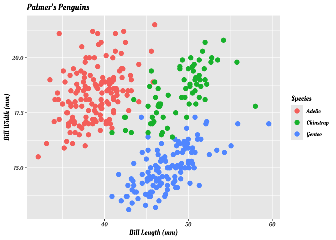
Let’s set up a basic scatterplot to start from:

Out of the box, the default ggplot theme uses pretty boring fonts. How might we change that?

In ggplot, the theme() function lets us control the appearance of various aspects of the plot. There are many, many properties we can tweak; we will begin by setting the global text property for all text on the entire plot.

Let’s try changing that font a bit:

demo_plt + theme(text=element_text(family="Optima"))

demo_plt + theme(text=element_text(family="Palatino"))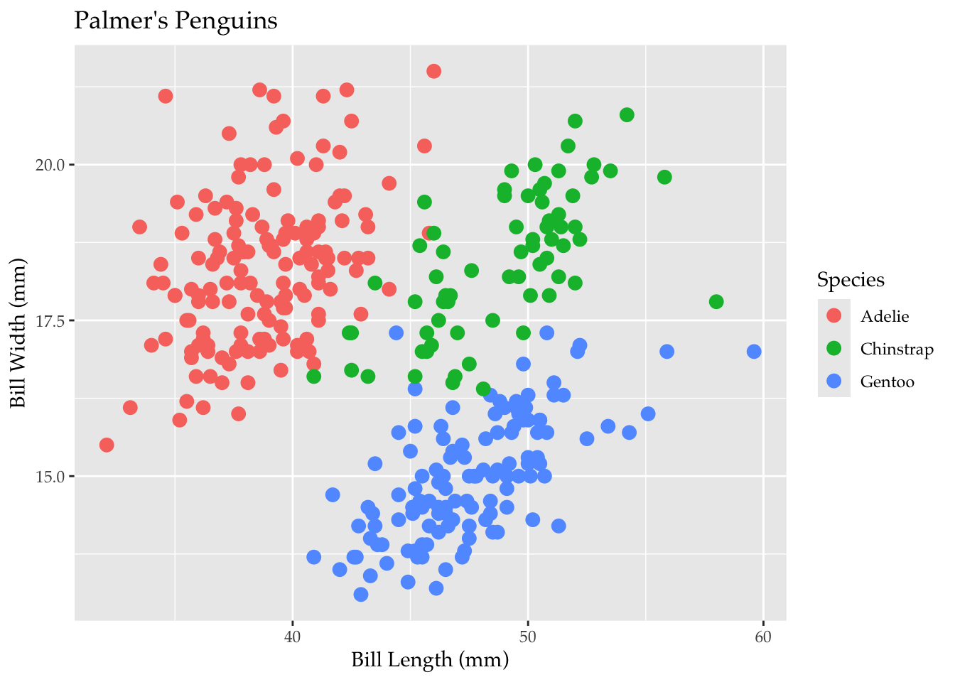

demo_plt + theme(text=element_text(family="Zapfino"))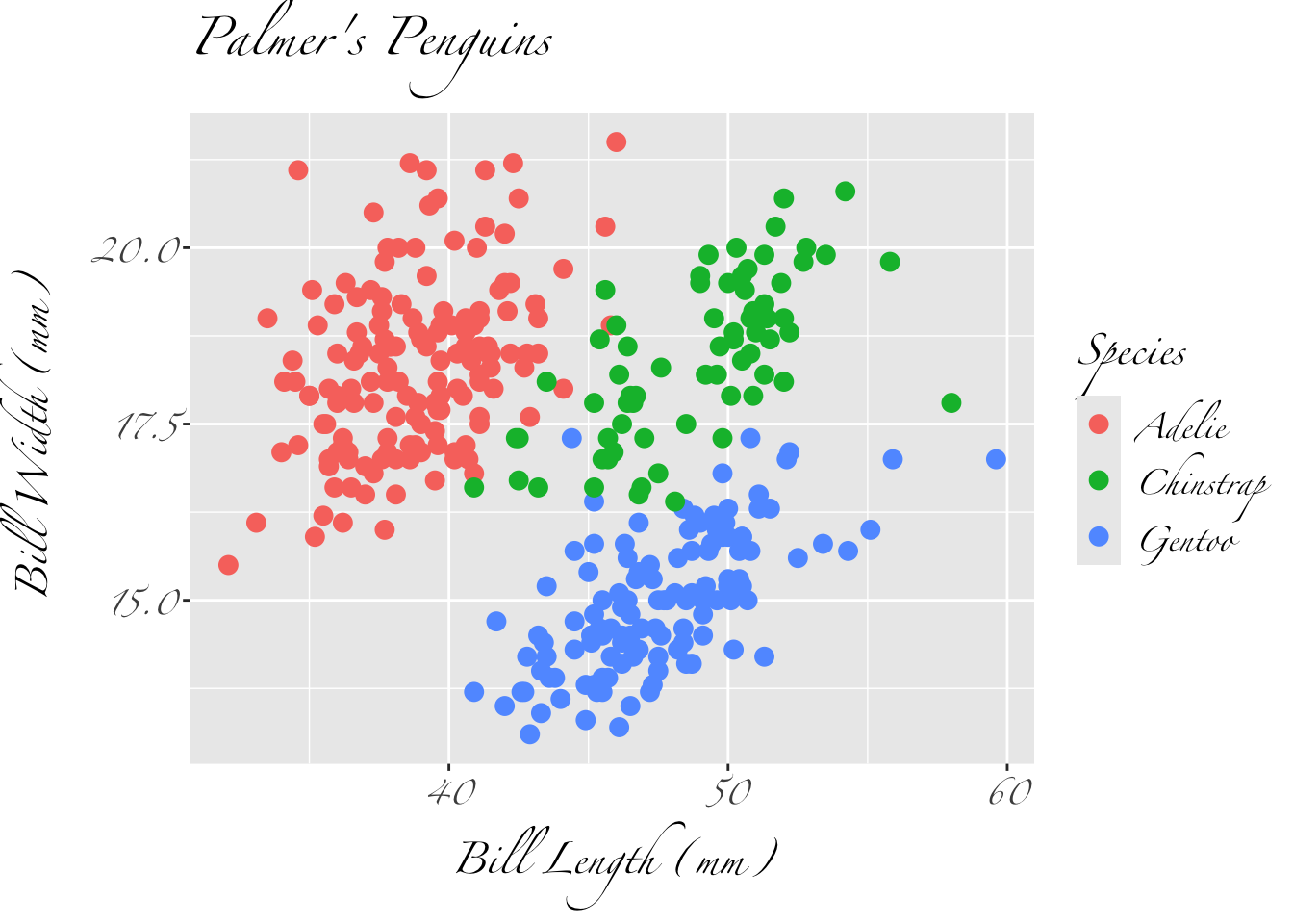

Note that the specific name that you must use to refer to the font is not exactly obvious. It is not the font name, but rather the font’s “family name”. Because of some under-the-hood details about the way that fonts work, this is a bit different from what you might see in e.g. a font selection menu in Word. You can see a list of all the fonts that R knows about by using the fonttable() command:

fonttable() %>% glimpse()

Rows: 296
Columns: 10
$ package    <lgl> NA, NA, NA, NA, NA, NA, NA, NA, NA, NA, NA, NA, NA, NA, NA, NA, NA, NA, NA, NA, NA, NA, NA, NA, NA, NA, NA, NA, NA, NA, …
$ afmfile    <chr> "SFCompactRounded.afm.gz", "Keyboard.afm.gz", "NewYork.afm.gz", "NewYorkItalic.afm.gz", "SFArabic.afm.gz", "SFCompact.af…
$ fontfile   <chr> "/System/Library/Fonts/SFCompactRounded.ttf", "/System/Library/Fonts/Keyboard.ttf", "/System/Library/Fonts/NewYork.ttf",…
$ FullName   <chr> ".SF Compact Rounded", ".Keyboard", ".New York", ".New York Italic", ".SF Arabic", ".SF Compact", ".SF Compact", "System…
$ FamilyName <chr> ".SF Compact Rounded", ".Keyboard", ".New York", ".New York", ".SF Arabic", ".SF Compact", ".SF Compact", "System Font",…
$ FontName   <chr> "--SFCompactRounded-Regular", "-Keyboard", "-NewYork-Regular", "-NewYork-RegularItalic", "-SFArabic-Regular", "-SFCompac…
$ Bold       <lgl> FALSE, FALSE, FALSE, FALSE, FALSE, FALSE, FALSE, FALSE, FALSE, FALSE, FALSE, FALSE, FALSE, FALSE, FALSE, FALSE, FALSE, F…
$ Italic     <lgl> FALSE, FALSE, FALSE, TRUE, FALSE, FALSE, TRUE, FALSE, TRUE, FALSE, TRUE, FALSE, FALSE, FALSE, FALSE, FALSE, FALSE, FALSE…
$ Symbol     <lgl> FALSE, FALSE, FALSE, FALSE, FALSE, FALSE, FALSE, FALSE, FALSE, FALSE, FALSE, FALSE, FALSE, FALSE, FALSE, FALSE, FALSE, F…
$ afmsymfile <lgl> NA, NA, NA, NA, NA, NA, NA, NA, NA, NA, NA, NA, NA, NA, NA, NA, NA, NA, NA, NA, NA, NA, NA, NA, NA, NA, NA, NA, NA, NA, …

fonttable() %>% head()

afmfile	fontfile	FullName	FamilyName	FontName	Bold	Italic	Symbol
SFCompactRounded.afm.gz	/System/Library/Fonts/SFCompactRounded.ttf	.SF Compact Rounded	.SF Compact Rounded	--SFCompactRounded-Regular	FALSE	FALSE	FALSE
Keyboard.afm.gz	/System/Library/Fonts/Keyboard.ttf	.Keyboard	.Keyboard	-Keyboard	FALSE	FALSE	FALSE
NewYork.afm.gz	/System/Library/Fonts/NewYork.ttf	.New York	.New York	-NewYork-Regular	FALSE	FALSE	FALSE
NewYorkItalic.afm.gz	/System/Library/Fonts/NewYorkItalic.ttf	.New York Italic	.New York	-NewYork-RegularItalic	FALSE	TRUE	FALSE
SFArabic.afm.gz	/System/Library/Fonts/SFArabic.ttf	.SF Arabic	.SF Arabic	-SFArabic-Regular	FALSE	FALSE	FALSE
SFCompact.afm.gz	/System/Library/Fonts/SFCompact.ttf	.SF Compact	.SF Compact	-SFCompact-Black	FALSE	FALSE	FALSE

fonttable() %>% select(FullName, FamilyName, FontName) %>% head(20)

FullName	FamilyName	FontName
.SF Compact Rounded	.SF Compact Rounded	--SFCompactRounded-Regular
.Keyboard	.Keyboard	-Keyboard
.New York	.New York	-NewYork-Regular
.New York Italic	.New York	-NewYork-RegularItalic
.SF Arabic	.SF Arabic	-SFArabic-Regular
.SF Compact	.SF Compact	-SFCompact-Black
.SF Compact	.SF Compact	-SFCompact-BlackItalic
System Font	System Font	-SFNS-Regular
System Font Regular Italic	System Font	-SFNS-RegularItalic
.SF NS Mono Light	.SF NS Mono	-SFNSMono-Light
.SF NS Mono Light Italic	.SF NS Mono	-SFNSMono-LightItalic
.SF NS Rounded	.SF NS Rounded	-SFNSRounded-Regular
Academy Engraved LET Plain:1.0	Academy Engraved LET	AcademyEngravedLetPlain
Andale Mono	Andale Mono	AndaleMono
Apple Braille	Apple Braille	AppleBraille
Apple Braille Outline 6 Dot	Apple Braille	AppleBraille-Outline6Dot
Apple Braille Outline 8 Dot	Apple Braille	AppleBraille-Outline8Dot
Apple Braille Pinpoint 6 Dot	Apple Braille	AppleBraille-Pinpoint6Dot
Apple Braille Pinpoint 8 Dot	Apple Braille	AppleBraille-Pinpoint8Dot
AppleMyungjo Regular	AppleMyungjo	AppleMyungjo

fonttable() %>% select(FamilyName) %>% distinct()

FamilyName
.SF Compact Rounded
.Keyboard
.New York
.SF Arabic
.SF Compact
System Font
.SF NS Mono
.SF NS Rounded
Academy Engraved LET
Andale Mono
Apple Braille
AppleMyungjo
Arial Black
Arial
Arial Narrow
Arial Rounded MT Bold
Arial Unicode MS
Atkinson Hyperlegible
Bitter
Bodoni Ornaments
Bodoni 72 Smallcaps

Brush Script MT
Calibri
Calibri Light
Charis SIL
Comic Sans MS
Consolas
Courier New
DIN Alternate
DIN Condensed
Doulos SIL
Fira Sans Black
Fira Sans
Fira Sans ExtraBold
Fira Sans ExtraLight
Fira Sans Light
Fira Sans Medium
Fira Sans SemiBold
Fira Sans Thin
Fondamento
Georgia
Gorni
Harding Text Web Bold
Harding Text Web Regular
HK Grotesk Black
HK Grotesk
HK Grotesk ExtraBold
HK Grotesk ExtraLight
HK Grotesk Light
HK Grotesk Medium
HK Grotesk SemiBold
HK Grotesk Thin
Impact
Karla
Khmer Sangam MN
Lao Sangam MN
Lato Black
Lato
Lato Hairline
Lato Light
Luminari
Microsoft Sans Serif
Noto Sans
Noto Sans Adlam
Noto Sans Avestan
Noto Sans Bamum
Noto Sans Bassa Vah
Noto Sans Batak
Noto Sans Bhaiksuki
Noto Sans Brahmi
Noto Sans Buginese
Noto Sans Buhid
Noto Sans Carian
Noto Sans CaucAlban
Noto Sans Chakma
Noto Sans Cham
Noto Sans Coptic
Noto Sans Cuneiform
Noto Sans Cypriot
Noto Sans Duployan
Noto Sans EgyptHiero
Noto Sans Elbasan
Noto Sans Glagolitic
Noto Sans Gothic
Noto Sans HanifiRohg
Noto Sans Hanunoo
Noto Sans Hatran
Noto Sans ImpAramaic
Noto Sans InsPahlavi
Noto Sans InsParthi
Noto Sans Kaithi
Noto Sans Kayah Li
Noto Sans Kharoshthi
Noto Sans Khojki
Noto Sans Khudawadi
Noto Sans Lepcha
Noto Sans Limbu
Noto Sans Linear A
Noto Sans Linear B
Noto Sans Lisu
Noto Sans Lycian
Noto Sans Lydian
Noto Sans Mahajani
Noto Sans Mandaic
Noto Sans Manichaean
Noto Sans Marchen
Noto Sans MeeteiMayek
Noto Sans Mende Kikakui
Noto Sans Meroitic
Noto Sans Miao
Noto Sans Modi
Noto Sans Mongolian
Noto Sans Mro
Noto Sans Multani
Noto Sans Nabataean
Noto Sans Newa
Noto Sans NewTaiLue
Noto Sans NKo
Noto Sans Ol Chiki
Noto Sans OldHung
Noto Sans Old Italic
Noto Sans OldNorArab
Noto Sans Old Permic
Noto Sans OldPersian
Noto Sans OldSouArab
Noto Sans Old Turkic
Noto Sans Osage
Noto Sans Osmanya
Noto Sans Pahawh Hmong
Noto Sans Palmyrene
Noto Sans PauCinHau
Noto Sans PhagsPa
Noto Sans Phoenician
Noto Sans PsaPahlavi
Noto Sans Rejang
Noto Sans Samaritan
Noto Sans Saurashtra
Noto Sans Sharada
Noto Sans Siddham
Noto Sans SoraSomp
Noto Sans Sundanese
Noto Sans Syloti Nagri
Noto Sans Syriac
Noto Sans Tagalog
Noto Sans Tagbanwa
Noto Sans Tai Le
Noto Sans Tai Tham
Noto Sans Tai Viet
Noto Sans Takri
Noto Sans Thaana
Noto Sans Tifinagh
Noto Sans Tirhuta
Noto Sans Ugaritic
Noto Sans Vai
Noto Sans Wancho
Noto Sans WarangCiti
Noto Sans Yi
Noto Serif
Noto Serif Ahom
Noto Serif Balinese
Open Sans
Open Sans Extrabold
Open Sans Light
Open Sans Semibold
Party LET
Pontano Sans
Pontano Sans Light
Pontano Sans Medium
Pontano Sans SemiBold
SF Compact
SF Pro
Tahoma
Tangerine
Times New Roman
Trattatello
Trebuchet MS
Verdana
Webdings
WeePeople
Wingdings
Wingdings 2
Wingdings 3
.SF Camera
.SF Arabic Rounded
.SF Armenian
.SF Armenian Rounded
.SF Georgian
.SF Georgian Rounded
.SF Hebrew
.SF Hebrew Rounded
Noto Serif Hmong Nyiakeng
STIX Two Text

Long story short, you’ll want to use the value in FamilyName to refer to your font of interest.

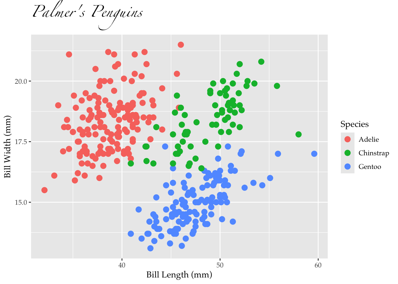
What if we wanted to have a different font for the title? The plot.title property is where we would want to look:

demo_plt + theme(
  text=element_text(family="Palatino"),
  plot.title=element_text(family="Zapfino")
  )

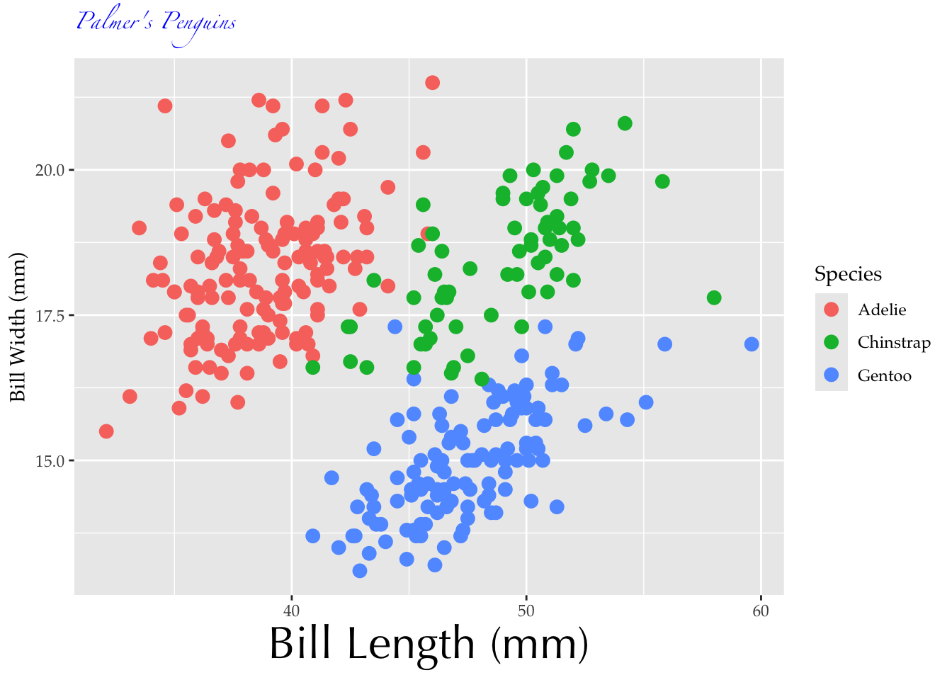
We can follow this pattern to change anything we like about the text in different parts of the plot:

demo_plt + theme(
  text=element_text(family="Palatino"),
  plot.title=element_text(family="Zapfino", size=8, color="blue"),
  axis.title.x = element_text(family="Optima", size=24)
  )

8.2 Installing new fonts

This part is a bit beyond the scope of this class, but the upshot is that after you install new fonts in your computer, you should tell extrafont about it using the font_import() command.

8.3 OTF Fonts:

extrafont only knows about TrueType fonts (ones whose file ends in .ttf); that’s why fonttable()’s output is missing so many fonts on my system. If you have an OpenType font you want to use with R, your best bet probably involves the showtext package.

You’ll need to know the exact filename of the font you want to add; on a Mac, you can use the built-in FontBook application to help you find this:

library(showtext)
font_add("Sofa Sans Regular", "FaceType - SofaSansHand-Regular.otf") # register the OTF font

Then, you just refer to it in your element_text() like any other font:

demo_plt + theme(
  text=element_text(family="Sofa Sans")
)

8.4 Using Google Fonts

showtext also has utility functions for working with Google Fonts. Google Fonts provides a wide variety of freely-usable font families, and is an amazing resource.

Here, we install and use the “Oleo Script” font.

font_add_google("Oleo Script")
showtext_auto() # For Google Fonts specifically, showtext may need this
demo_plt + theme(
  text=element_text(family="Oleo Script")
)

8.5 A Caveat and a Plea

It is important to note that both extrafont and showtext work best for raster images; there are certain quirks that you are likely to encounter when producing PDF output using non-standard fonts (or, depending on the font, a plot that uses text containing text from the non-BMP regions of Unicode, like emojis). The story of “making PDFs with non-standard fonts in R” is extremely long and tedious; if you are actually interested, set up a meeting and I will be happy to go over it with you.

The upshot of it all is that if you want to make a PDF from ggplot using non-standard fonts or with non-BMP Unicode characters, your best bet is to use showtext, which will produce a perfectly nice PDF file with whatever font and text you want… with one caveat: text selection (for search, copy-and-paste, etc.) will not be possible in the resulting PDFs. The file will look fine for everybody, it will print fine for everybody, it will scale fine to any resolution, and will do all the things a PDF should do, other than allow text extraction.

If this is a dealbreaker for your particular situation, my honest advice is to find a different font to use- pick a TTF font (or figure out how to convert your OTF font to a TTF font), use extrafont, and move on with your life. Life is short and fleeting, the grave is cold and lonely, the climate is changing, and the full day that you will spend debugging this situation is a day of your life that you can never get back. Nobody, on their deathbed, has ever wished that they had spent more time debugging mysterious error messages involving multiple obscure pieces of thirty-five-year-old software in order to get a PDF file to behave slightly better. Please, spend that day with your family, or go enjoy the coastline while it’s still there, or do literally anything else other than try and get R to produce proper PDF output with OTF fonts.

And note that this is advice coming from somebody who actually enjoys dealing with bizarre font and Unicode issues, is a perfectionist when it comes to fonts and PDF files, and who eventually decided to acknowledge reality and just use showtext.

If you absolutely must ignore my advice, here are two places to start:

Section 14.6 of the R Graphics Cookbook
My own page on the subject, which includes some more detailed discussion and a workaround for what is going wrong with PDFs made using extrafont and non-standard TTF fonts
- Note that this page will offer neither advice nor solace for those suffering from the OTF font situation

Lab 05: Fonts & Tables

BMI 5/625

Alison Hill & Steven Bedrick

1 Goals for Lab 05

2 TL;DR

3 `knitr::kable`

3.1 `kable` all tables everywhere

3.2 `kable` table in a chunk

3.3 Styled `kable` tables in a chunk

3.4 Controlling column appearance

3.5 `kable` + `kableExtra` + `formattable`

3.6 `tibble` + `kable` + `kableExtra`

4 Markdown Tables

4.1 Simple table

4.2 Multi-line tables

4.3 Grid tables

4.4 Pipe tables

5 `gt`

6 Descriptive Stats tables

6.1 `tableone`

6.2 `table1`

7 The `DT` package

8 Finally, fonts!

8.1 Your friend, `extrafont`

8.2 Installing new fonts

8.3 OTF Fonts:

8.4 Using Google Fonts

8.5 A Caveat and a Plea

Lab 05: Fonts & Tables

BMI 5/625

Alison Hill & Steven Bedrick

1 Goals for Lab 05

2 TL;DR

3 knitr::kable

3.1 kable all tables everywhere

3.2 kable table in a chunk

3.3 Styled kable tables in a chunk

3.4 Controlling column appearance

3.5 kable + kableExtra + formattable

3.6 tibble + kable + kableExtra

4 Markdown Tables

4.1 Simple table

4.2 Multi-line tables

4.3 Grid tables

4.4 Pipe tables

5 gt

6 Descriptive Stats tables

6.1 tableone

6.2 table1

7 The DT package

8 Finally, fonts!

8.1 Your friend, extrafont

8.2 Installing new fonts

8.3 OTF Fonts:

8.4 Using Google Fonts

8.5 A Caveat and a Plea

3 `knitr::kable`

3.1 `kable` all tables everywhere

3.2 `kable` table in a chunk

3.3 Styled `kable` tables in a chunk

3.5 `kable` + `kableExtra` + `formattable`

3.6 `tibble` + `kable` + `kableExtra`

5 `gt`

6.1 `tableone`

6.2 `table1`

7 The `DT` package

8.1 Your friend, `extrafont`