Lab 07: Interactive Vis With Shiny
BMI 5/625
Steven Bedrick
1 Introduction
Shiny is a powerful R library for making interactive web sites containing visualizations and tables. In this lab, you will learn the basics of designing and building a simple interactive dashboard for exploring a data set. Since the final product of a Shiny application is a web site, much of what you learned in the last lab will be useful this week!
1.1 Getting Started
To begin, install and load the shiny library. We’ll also load the tidyverse:
library(shiny)
library(tidyverse)
In the last lab, we learned about static web site. Under this model, the web site consists of a collection of HTML files (along with images, etc.); the user, via their web browser, requests those files from a server. The server’s role is to find the requested file, and then send it back to the browser (the response).
A Shiny application is an example of a dynamic website. The first part of the process is the same: the user interacts with the web site via their browser, and the results of their interactions (links or buttons clicked, form fields filled out, etc.) are sent to the server in the form of a request. The server’s role is quite different under a dynamic scenario. Instead of simply finding a static page and returning it, the server instead executes a program (specified in the request), and sends the results of that program back to the browser as the response.
The results often take the form of rendered HTML. That is to say, HTML that is dynamically generated in response to the user’s actions and input, rather than loaded directly from a file on disk. In a Shiny application, this takes the form of an R program.
Shiny applications divide their world between a front end, the user interface that the browser displays, and the back end, the chunks of R code that are run in response to user actions.
1.2 First step with shiny:
The structure of a shiny application is simple. You’ll need a file called app.R, with three main pieces.
- Code describing the front end: what text goes where, what buttons are present, etc.
- Code describing the back end: what should happen in response to user activities, and how to compute figures, tables, etc.
- A call to the
shinyApp()function, to actually run your application
Here is a simple app.R:
library(shiny)
ui <- fluidPage(
titlePanel("Hello, world!"),
"This is some text!"
)
server <- function(input, output, session) {
# nothing to do here, for now
}
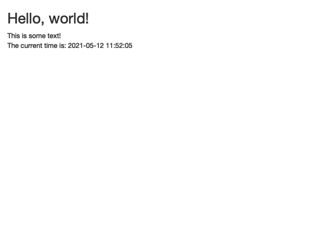
shinyApp(ui = ui, server = server)Try putting this in your app.R and run it. You should see something like this:

Note above the titlePanel() function. This is a function whose output is HTML:
titlePanel("Hello, world!")[1] "<h2>Hello, world!</h2>"We’ll see that Shiny includes a variety of other functions for controlling the HTML that goes in to our UI.
2 Make it dynamic
This is a complete application, but it doesn’t do anything interesting. Let’s make it a bit more interesting, and have it print the date and time that the page was loaded.
There are a few new pieces here:
- We have added a
textOutputelement to our UI; - Assigned it the name
timestamp, and - In the
serverfunction, we are callingrenderText()to populate it:
library(shiny)

ui <- fluidPage(
  titlePanel("Hello, world!"),
  "This is some text!",
  textOutput("timestamp"),
)

server <- function(input, output, session) {

  output$timestamp <- renderText({
      paste0("The current time is: ", Sys.time())
    })
}

shinyApp(ui = ui, server = server)
There are corresponding *Output elements (and render*() functions) for images, plots, tables, etc. We’ll see examples of that as we move forward.
The other important thing to notice in this example is that we are giving our UI element an identifier, “timestamp”, which we use later in the server function:
library(shiny)

ui <- fluidPage(
  titlePanel("Hello, world!"),
  "This is some text!",
  textOutput("timestamp"),
)

server <- function(input, output, session) {

  output$timestamp <- renderText({
      paste0("The current time is: ", Sys.time())
    })
}

shinyApp(ui = ui, server = server)
This is a key pattern in Shiny. A way to think about it is that the element IDs are links that let the front-end and back-end communicate with one another. When you run this application, you should see something like this:
2.1 Collecting User Input
We frequently want to collect input from our user (for example, to specify which data set to visualize, set the title of a plot, a value to filter by, etc.). Shiny makes this easy. Our next application will ask the user for their name, and then tell us how long their name is. (This is kind of a silly example, but will illustrate how to capture user-entered info). Let us begin with the UI:
library(shiny)

ui <- fluidPage(
  titlePanel("Name Measurement"),
  textInput("name", label="What is your name?"),
  textOutput("nameLength")
)

server <- function(input, output, session) {
}

shinyApp(ui = ui, server = server)
We have added a new element: textInput. This is one of the many *input() elements, corresponding to things like text boxes, drop-down menus, date pickers, sliders (for entering numeric values), etc. (See the Shiny Widgets Gallery for examples of each of the available controls).
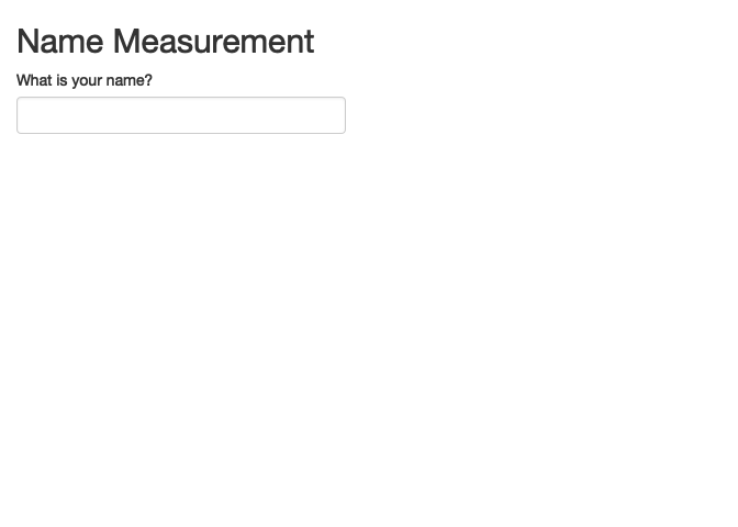
When we run this application, we should see something like this:
How might we access the value of our name field from the back-end? To set a value in the UI, we used the output variable; to get a value from the UI, we use the input variable. We will use stringr’s str_length() function, and send its output back via renderText():
server <- function(input, output, session) {
  output$nameLength <- renderText(
      paste0("Your name is ", str_length(input$name), " letters long.")
    )
}
Try adding this line to your server function, and run the application. You should see something like this:
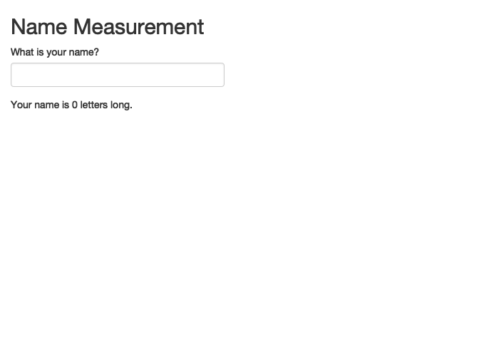
What happens if you type your name in the text box?
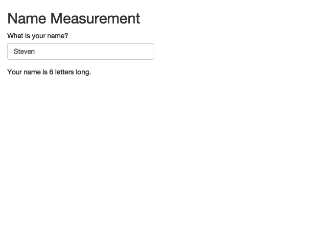
Note that the contents of the UI automatically updates when fields change. Shiny uses a reactive programming model, in which elements on the page automatically react to one another.
Another thing to note here is that we are providing textInput with a default value (“Steven”, in this case). What happens if we don’t do this?
2.2 Including a plot
Let’s do something more interesting than just showing the length of a name; let’s instead show a plot, using data from the babynames package. The plot will be a simple line plot for a particular name, split by sex:
babynames %>%
            filter(name=="Steven") %>%
            ggplot(mapping=aes(x=year, y=prop, color=sex)) +
            geom_line() +
            ggtitle("Name Frequency: Steven")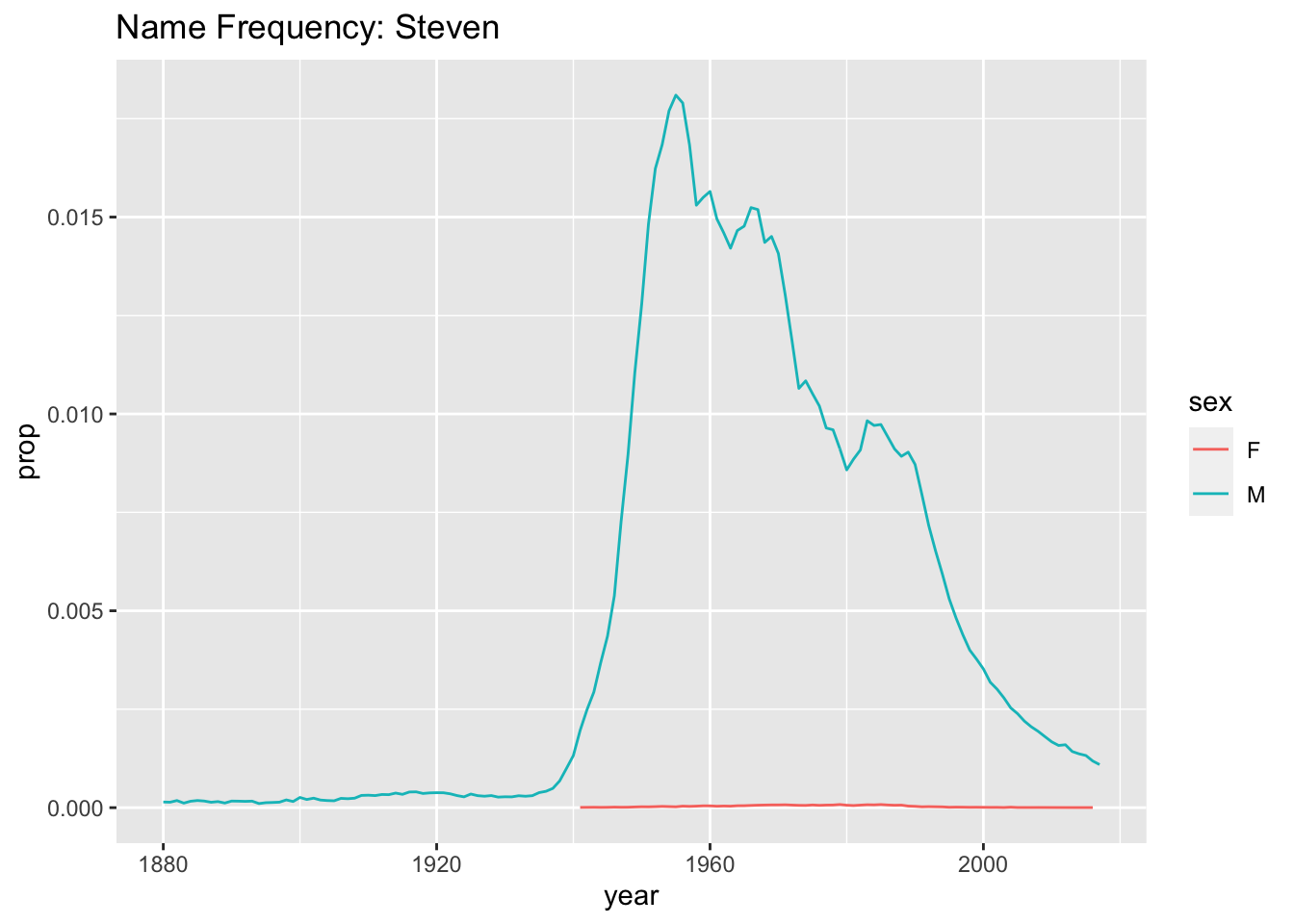
Nothing fancy, but that’s fine- let’s get it into our Shiny application. We will use the plotOutput/renderPlot functions:
library(shiny)
library(babynames)

ui <- fluidPage(
  titlePanel("Name Measurement"),
  textInput("name", label="What is your name?", value="Steven"),
  plotOutput("namePlot")
)

server <- function(input, output, session) {
    output$namePlot <- renderPlot({
        babynames %>%
            filter(name==input$name) %>%
            ggplot(mapping=aes(x=year, y=prop, color=sex)) +
            geom_line() +
            ggtitle(paste0("Name Frequency: ", input$name))
    })
}

shinyApp(ui = ui, server = server)
plotOutput can take display figures made with either plot() or ggplot().
Note that we are now providing the name text box a default value, so that the page has something to show when it first loads. What happens if you take that out?
Also note that our renderPlot() call is using curly-braces, so that we can give it multiple lines of input.
2.3 Including a table
In addition to a plot, let’s also include a little data table showing the year in which the name in question was most popular. Our code to generate the table will look like this:
babynames %>%
  filter(name=="Steven") %>%
  group_by(sex) %>%
  arrange(year) %>%
  top_n(1, prop) %>%
  select(-name)
# A tibble: 2 x 4
# Groups: sex [2]
year sex n prop
<dbl> <chr> <int> <dbl>
1 1955 M 37816 0.0181
2 1979 F 137 0.0000795As you might imagine, Shiny has an tableOutput()/renderTable() pair:
library(shiny)
library(babynames)

ui <- fluidPage(
  titlePanel("Name Measurement"),
  textInput("name", label="What is your name?", value="Steven"),
  plotOutput("namePlot"),
  tableOutput("nameTable")
)

server <- function(input, output, session) {
    output$namePlot <- renderPlot({
        babynames %>%
            filter(name==input$name) %>%
            ggplot(mapping=aes(x=year, y=prop, color=sex)) +
            geom_line() +
            ggtitle(paste0("Name Frequency: ", input$name))
    })

    output$nameTable <- renderTable({
      babynames %>%
        filter(name==input$name) %>%
        group_by(sex) %>%
        arrange(year) %>%
        top_n(1, prop) %>%
        select(-name)

    })
}

shinyApp(ui = ui, server = server)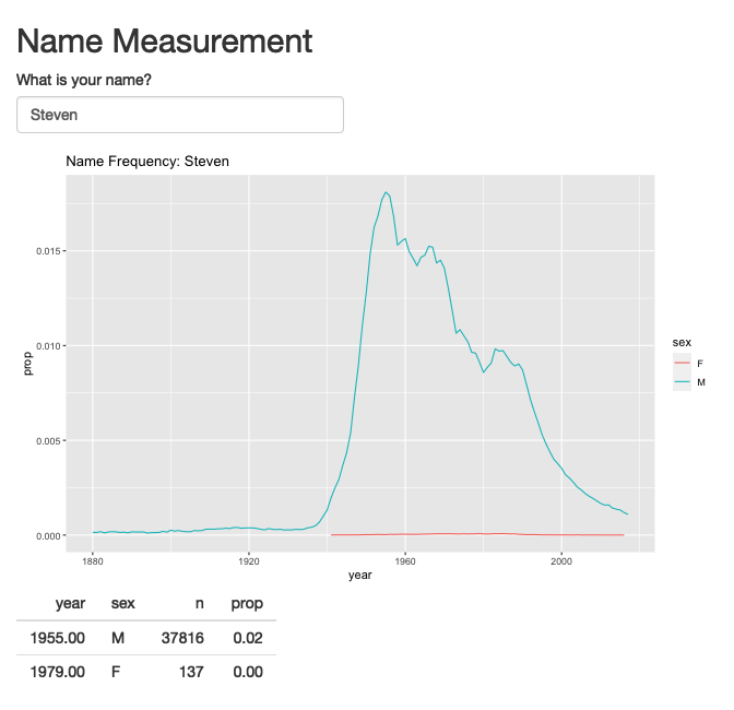
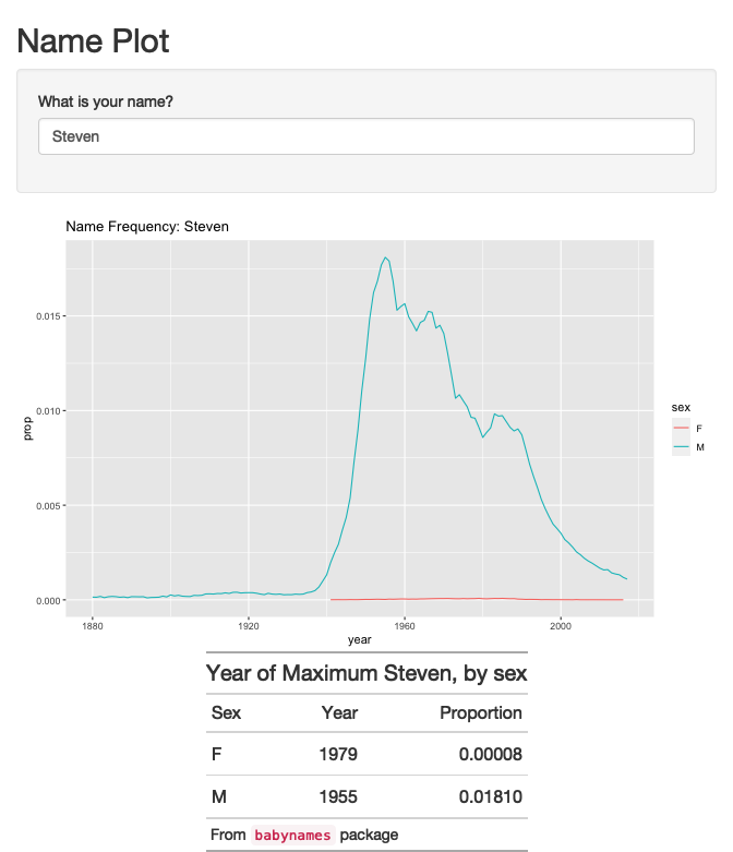
This is kind of basic-looking, but can be customized as much as one might wish, using any of the table formatting techniques we discussed earlier in the term. Notably, the gt package includes some special Shiny-related functions. Here’s a fancier version of the table from above:
babynames %>%
        filter(name=="Steven") %>%
        group_by(sex) %>%
        arrange(year) %>%
        top_n(1, prop) %>%
        select(-name) %>% ungroup() %>% select(sex, year, prop) %>%
        arrange(sex) %>%
  gt() %>%
    cols_label(sex="Sex", year="Year", prop="Proportion") %>%
    fmt_number(columns=c(prop), decimals=5) %>%
    tab_header(title="Year of Maximum Steven, by sex")  %>%
tab_source_note(md("From `babynames` package"))| Year of Maximum Steven, by sex | ||
|---|---|---|
| Sex | Year | Proportion |
| F | 1979 | 0.00008 |
| M | 1955 | 0.01810 |
From babynames package |
||
We can integrate that into our Shiny display using gt’s render_gt() and gt_output() functions:
library(shiny)
library(babynames)
library(gt)

ui <- fluidPage(
  titlePanel("Name Measurement"),
  textInput("name", label="What is your name?", value="Steven"),
  plotOutput("namePlot"),
  gt_output("nameTable")
)

server <- function(input, output, session) {
    output$namePlot <- renderPlot({
        babynames %>%
            filter(name==input$name) %>%
            ggplot(mapping=aes(x=year, y=prop, color=sex)) +
            geom_line() +
            ggtitle(paste0("Name Frequency: ", input$name))
    })

    output$nameTable <- render_gt({
    babynames %>%
        filter(name==input$name) %>%
        group_by(sex) %>%
        arrange(year) %>%
        top_n(1, prop) %>%
        select(-name) %>% ungroup() %>% select(sex, year, prop) %>%
        arrange(sex) %>%
    gt() %>%
      cols_label(sex="Sex", year="Year", prop="Proportion") %>%
      fmt_number(columns=c(prop), decimals=5) %>%
      tab_header(title=paste0("Year of Maximum ", input$name, ", by sex"))  %>%
      tab_source_note(md("From `babynames` package"))

    })
}

shinyApp(ui = ui, server = server)
3 Organizing our app
At this point, our server function is getting a bit unruly. A good practice is to encapsulate various parts of the display into separate functions, like so:
library(shiny)
library(babynames)
library(gt)

makePlot <- function(nameToUse) {
  babynames %>%
            filter(name==nameToUse) %>%
            ggplot(mapping=aes(x=year, y=prop, color=sex)) +
            geom_line() +
            ggtitle(paste0("Name Frequency: ", nameToUse))
}

makeTable <- function(nameToUse) {
  babynames %>%
        filter(name==nameToUse) %>%
        group_by(sex) %>%
        arrange(year) %>%
        top_n(1, prop) %>%
        select(-name) %>% ungroup() %>% select(sex, year, prop) %>%
        arrange(sex) %>%
    gt() %>%
      cols_label(sex="Sex", year="Year", prop="Proportion") %>%
      fmt_number(columns=c(prop), decimals=5) %>%
      tab_header(title=paste0("Year of Maximum ", nameToUse, ", by sex"))  %>%
      tab_source_note(md("From `babynames` package"))
}

ui <- fluidPage(
  titlePanel("Name Measurement"),
  textInput("name", label="What is your name?", value="Steven"),
  plotOutput("namePlot"),
  gt_output("nameTable")
)

server <- function(input, output, session) {
    output$namePlot <- renderPlot(makePlot(input$name))

    output$nameTable <- render_gt(makeTable(input$name))
}

shinyApp(ui = ui, server = server)
Note that the functions that make the plot and the table do not directly reference the input variable provided by Shiny- they would work just fine “one their own”, independent of whether we were using Shiny or not. Similarly, the parts of the application responsible for handling input and output via Shiny (i.e., textInput, renderPlot) do not need to concern themselves with the details of what might be involved in generating the plots, etc.
This is an example of decoupling the different parts of our application from one another: the code to generate the tables and plots can be written and tested independently of the parts of the program that are , and as a result changes that we make to one part will (hopefully) not have any impact on the other parts.
4 Customizing the layout
Visually, the layout of our page is starting to get a bit long; what if we wanted to arrange it so that the plot and the table were side-by-side? Shiny gives us many options for controlling the layout; the simplest is to arrange things in rows and columns. Shiny uses the “Bootstrap” CSS library, which is built around a 12-column layout. We can use the fluidRow() and column() functions to set things up a bit differently:
ui <- fluidPage(
  titlePanel("Name Measurement"),
  textInput("name", label="What is your name?", value="Steven"),
  fluidRow(
    column(6, plotOutput("namePlot")),
    column(6, gt_output("nameTable"))
  )
)
Between fluidRow() and column(), you can put together pretty much any layout you might want, but a useful shortcut may be to use the sidebarLayout() function:
ui <- fluidPage(
  titlePanel("Name Plot"),
  sidebarLayout(
    sidebarPanel(
      textInput("name", label="What is your name?", value="Steven")
    ),
    mainPanel(
      plotOutput("namePlot"),
      gt_output("nameTable")
    )
  )
)
sidebarLayout() is one of several built-in layout helper functions in Shiny, and can be used to quickly build a more complex interface. Note that in the screenshot below, our “sidebar” is actually being placed above the plot; in reality, pages using sidebarLayout will be responsive to the window size in which they are viewed. In a narrower window (or on a phone) it will automatically reflow to a vertical layout.
5 Other controls
5.2 Getting Fancy: observeEvent
Now let’s make the system more powerful. In the above example, I have set the list of names to be the top 10 names from 2017. Let’s allow the user to specify a year, using numericInput. This will involve a few new concepts, specifically around linking the value of one field to the value of another. First, let’s look at the UI:
ui <- fluidPage(
    titlePanel("Name Measurement"),
    numericInput("year", label="Year", min=1880, max=2017, value=2017),
    selectInput("name", label="Which Name?", c()),
    fluidRow(
        column(6, plotOutput("namePlot")),
        column(6, gt_output("nameTable"))
    )
)
We’ve added a new input control, which will only allow numeric input that is within a certain range. We’ve also stopped manually specifying our select box options, since we want the list to be dynamic: it should contain the top ten names for the selected year. We need to somehow connect the numericInput box that we have created to the selectInput. We’ll do this in the server function:
server <- function(input, output, session) {

    namesToUse <- reactive({
        babynames %>%
            filter(year==input$year) %>%
            group_by(sex) %>%
            arrange(prop) %>% top_n(5) %>%
            ungroup() %>% select(name)
    })

    observeEvent(namesToUse(), {
        updateSelectInput(session, "name",
                          choices=namesToUse(),
                          label=paste0("Popular names in ", input$year)
                          )
    })

    # note: don't forget the code to actually make the plot and table!

}
There are two new things here. First is the use of the reactive() function, which sets up a new variable that Shiny will be in charge of. Any R variable that we want to either use or be used by a Shiny component must be wrapped in a reactive() call. In this case, our list of names depends on (i.e., is using) input$year, so we have to make it reactive.
Try it out: What happens if we don’t wrap our code here in reactive()?
Once our list of common names has been made reactive, we can wire it up to other parts of the UI via observeEvent(). Code inside observeEvent() is run whenever the variable that it is connected to changes; in this case, upateSelectInput() will be run when a new year is entered. Pretty neat!
6 Deployment
See the shinyapps.io user guide for information about deploying a simple Shiny app.
7 Deliverable
For this week, you will construct and deploy a Shiny app that will let the user explore Kieran Healy’s covdata package containing up-to-date COVID-19 data. There are a variety of interesting data sets in this package, including ; feel free to draw inspiration from some of his blog posts (under “Articles” on the covdata home page). Think about the kinds of visualization and analysis tasks that are well-supported by interactivity, and recall Shneiderman’s mantra (“Overview first, zoom and filter, then details on demand”) as you work.
I strongly recommend referring to the Shiny links on the syllabus for additional information and ideas!
![]()