Lab 05: Fonts & Tables

BMI 5/625

1 Goals for Lab 05

Become familiar with tools for generating publication-ready tables directly in R.

We will use data from the following paper: MacFarlane, H., Gorman, K., Ingham, R., Presmanes Hill, A., Papadakis, K., Kiss, G., & van Santen, J. (2017). Quantitative analysis of disfluency in children with autism spectrum disorder or language impairment. PLoS ONE, 12(3), e0173936.

mazes <- read_csv("http://bit.ly/mazes-gist") %>% 
  clean_names()  #janitor package

glimpse(mazes)

Rows: 381
Columns: 12
$ study_id <chr> "CSLU-001", "CSLU-001", "CSLU-001", "CSLU-001", "CSLU-002", "…
$ ca       <dbl> 5.6667, 5.6667, 5.6667, 5.6667, 6.5000, 6.5000, 6.5000, 6.500…
$ viq      <dbl> 124, 124, 124, 124, 124, 124, 124, 124, 108, 108, 108, 108, 1…
$ dx       <chr> "TD", "TD", "TD", "TD", "TD", "TD", "TD", "TD", "TD", "TD", "…
$ activity <chr> "Conversation", "Picture Description", "Play", "Wordless Pict…
$ content  <dbl> 24, 1, 21, 8, 3, 5, 8, 2, 25, 10, 2, 5, 32, 20, 13, 21, 27, 9…
$ filler   <dbl> 31, 2, 6, 2, 10, 3, 8, 2, 21, 13, 10, 2, 12, 9, 4, 4, 12, 6, …
$ rep      <dbl> 2, 0, 3, 0, 3, 2, 3, 0, 4, 0, 0, 0, 13, 5, 5, 6, 10, 5, 5, 2,…
$ rev      <dbl> 5, 0, 8, 4, 0, 1, 2, 0, 4, 2, 1, 3, 8, 7, 2, 8, 5, 1, 4, 2, 1…
$ fs       <dbl> 17, 1, 10, 4, 0, 2, 3, 2, 17, 8, 1, 2, 11, 8, 6, 7, 12, 3, 3,…
$ cued     <dbl> 36, 2, 6, 2, 10, 3, 9, 2, 29, 13, 11, 2, 14, 12, 4, 11, 17, 7…
$ not_cued <dbl> 50, 3, 27, 10, 13, 8, 15, 4, 38, 23, 11, 7, 42, 26, 17, 18, 3…

2 TL;DR

The workhorse for making tables in R Markdown documents is the knitr package’s kable function. This function is really versatile, but also free of fancy formatting options, for better or worse.

3 knitr::kable

3.1 kable all tables everywhere

In order to tell RMarkdown to use kable to format all tabular output, update the YAML of your document. For HTML:

---
title: "My Awesome Data Vis Lab"
output:
  html_document:
    df_print: kable
---

You can also define the html format in the global options.

# If you don't define format here, you'll need put `format = "html"` in every kable function.
options(knitr.table.format = "html") 
# You may also wish to set this option
options(scipen = 1, digits = 2)

3.2 kable table in a chunk

For HTML output:

head(mazes) %>% 
  kable(format = "html")

study_id	ca	viq	dx	activity	content	filler	rep	rev	fs	cued	not_cued
CSLU-001	5.6667	124	TD	Conversation	24	31	2	5	17	36	50
CSLU-001	5.6667	124	TD	Picture Description	1	2	0	0	1	2	3
CSLU-001	5.6667	124	TD	Play	21	6	3	8	10	6	27
CSLU-001	5.6667	124	TD	Wordless Picture Book	8	2	0	4	4	2	10
CSLU-002	6.5000	124	TD	Conversation	3	10	3	0	0	10	13
CSLU-002	6.5000	124	TD	Picture Description	5	3	2	1	2	3	8

Note that this is a bit rough-looking. We will use various features of kable to improve our output.

For starters, we can add a caption:

head(mazes) %>% 
  kable(format = "html", digits = 2, caption = "A table produced by kable.")

A table produced by kable.

study_id	ca	viq	dx	activity	content	filler	rep	rev	fs	cued	not_cued
CSLU-001	5.67	124	TD	Conversation	24	31	2	5	17	36	50
CSLU-001	5.67	124	TD	Picture Description	1	2	0	0	1	2	3
CSLU-001	5.67	124	TD	Play	21	6	3	8	10	6	27
CSLU-001	5.67	124	TD	Wordless Picture Book	8	2	0	4	4	2	10
CSLU-002	6.50	124	TD	Conversation	3	10	3	0	0	10	13
CSLU-002	6.50	124	TD	Picture Description	5	3	2	1	2	3	8

We can also manually specify human-readable column names:

my_maze_names <- c("Participant", "Age", "Verbal\nIQ", "Group", "Activity", "Content\nMaze", "Filler\nMaze", "Repetition", "Revision", "False\nStart", "Cued", "Not\nCued")
head(mazes) %>% 
  kable(format = "html", digits = 2, caption = "A table produced by kable.",
        col.names = my_maze_names)

A table produced by kable.

Participant	Age	Verbal IQ	Group	Activity	Content Maze	Filler Maze	Repetition	Revision	False Start	Cued	Not Cued
CSLU-001	5.67	124	TD	Conversation	24	31	2	5	17	36	50
CSLU-001	5.67	124	TD	Picture Description	1	2	0	0	1	2	3
CSLU-001	5.67	124	TD	Play	21	6	3	8	10	6	27
CSLU-001	5.67	124	TD	Wordless Picture Book	8	2	0	4	4	2	10
CSLU-002	6.50	124	TD	Conversation	3	10	3	0	0	10	13
CSLU-002	6.50	124	TD	Picture Description	5	3	2	1	2	3	8

3.3 Styled kable tables in a chunk

To improve the visual layout of the table, we can use the kableExtra package, which provides the kable_styling() function:

head(mazes) %>% 
  kable(format = "html", digits = 2, caption = "A styled kable table.",
        col.names = my_maze_names) %>% 
  kable_styling()

A styled kable table.

Participant	Age	Verbal IQ	Group	Activity	Content Maze	Filler Maze	Repetition	Revision	False Start	Cued	Not Cued
CSLU-001	5.67	124	TD	Conversation	24	31	2	5	17	36	50
CSLU-001	5.67	124	TD	Picture Description	1	2	0	0	1	2	3
CSLU-001	5.67	124	TD	Play	21	6	3	8	10	6	27
CSLU-001	5.67	124	TD	Wordless Picture Book	8	2	0	4	4	2	10
CSLU-002	6.50	124	TD	Conversation	3	10	3	0	0	10	13
CSLU-002	6.50	124	TD	Picture Description	5	3	2	1	2	3	8

There are lots of printing options: https://haozhu233.github.io/kableExtra/awesome_table_in_html.html

head(mazes) %>% 
  kable(format = "html", digits = 2, caption = "A non-full width zebra kable table.") %>% 
  kable_styling(bootstrap_options = "striped", full_width = F)

A non-full width zebra kable table.

study_id	ca	viq	dx	activity	content	filler	rep	rev	fs	cued	not_cued
CSLU-001	5.67	124	TD	Conversation	24	31	2	5	17	36	50
CSLU-001	5.67	124	TD	Picture Description	1	2	0	0	1	2	3
CSLU-001	5.67	124	TD	Play	21	6	3	8	10	6	27
CSLU-001	5.67	124	TD	Wordless Picture Book	8	2	0	4	4	2	10
CSLU-002	6.50	124	TD	Conversation	3	10	3	0	0	10	13
CSLU-002	6.50	124	TD	Picture Description	5	3	2	1	2	3	8

head(mazes) %>% 
  kable(format = "html", digits = 2, caption = "Over here!") %>% 
  kable_styling(bootstrap_options = "striped", full_width = F, position = "left")

Over here!

study_id	ca	viq	dx	activity	content	filler	rep	rev	fs	cued	not_cued
CSLU-001	5.67	124	TD	Conversation	24	31	2	5	17	36	50
CSLU-001	5.67	124	TD	Picture Description	1	2	0	0	1	2	3
CSLU-001	5.67	124	TD	Play	21	6	3	8	10	6	27
CSLU-001	5.67	124	TD	Wordless Picture Book	8	2	0	4	4	2	10
CSLU-002	6.50	124	TD	Conversation	3	10	3	0	0	10	13
CSLU-002	6.50	124	TD	Picture Description	5	3	2	1	2	3	8

3.4 Controlling column appearance

We can control the formatting of individual columns using the column_spec() function:

head(mazes) %>% 
  kable(format = "html", digits = 2, caption = "Over here!") %>% 
  kable_styling(bootstrap_options = "striped", full_width = F, position = "left") %>% 
  column_spec(4, width="3cm", background="lightblue", border_right=TRUE)

Over here!

study_id	ca	viq	dx	activity	content	filler	rep	rev	fs	cued	not_cued
CSLU-001	5.67	124	TD	Conversation	24	31	2	5	17	36	50
CSLU-001	5.67	124	TD	Picture Description	1	2	0	0	1	2	3
CSLU-001	5.67	124	TD	Play	21	6	3	8	10	6	27
CSLU-001	5.67	124	TD	Wordless Picture Book	8	2	0	4	4	2	10
CSLU-002	6.50	124	TD	Conversation	3	10	3	0	0	10	13
CSLU-002	6.50	124	TD	Picture Description	5	3	2	1	2	3	8

3.5 kable + kableExtra + formattable

color_tile and color_bar are neat extras if used wisely!

http://haozhu233.github.io/kableExtra/use_kableExtra_with_formattable.html

library(formattable)
head(mazes) %>% 
  mutate(ca = color_tile("transparent", "lightpink")(ca),
         viq = color_bar("lightseagreen")(viq)) %>%
  kable("html", escape = F, caption = 'This table is colored.') %>%
  kable_styling(position = "center") %>% 
  column_spec(4, width = "3cm") 

This table is colored.

study_id	ca	viq	dx	activity	content	filler	rep	rev	fs	cued	not_cued
CSLU-001	5.6667	124	TD	Conversation	24	31	2	5	17	36	50
CSLU-001	5.6667	124	TD	Picture Description	1	2	0	0	1	2	3
CSLU-001	5.6667	124	TD	Play	21	6	3	8	10	6	27
CSLU-001	5.6667	124	TD	Wordless Picture Book	8	2	0	4	4	2	10
CSLU-002	6.5000	124	TD	Conversation	3	10	3	0	0	10	13
CSLU-002	6.5000	124	TD	Picture Description	5	3	2	1	2	3	8

3.6 tibble + kable + kableExtra

You can also use any of these tools with plain text tables using the tibble package to create a table. Two main functions:

• tribble: enter tibble by rows
• tibble: enter tibble by columns

For example, I used tribble to make this table in our slide decks:

math_table <- tibble::tribble(
  ~Operator, ~Description, ~Usage,
  "\\+", "addition", "x + y",
  "\\-", "subtraction", "x - y",
  "\\*", "multiplication", "x * y",
  "/", "division", "x / y",
  "^", "raised to the power of", "x ^ y",
  "abs", "absolute value", "abs(x)",
  "%/%", "integer division", "x %/% y",
  "%%", "remainder after division", "x %% y"
)

Then I used this chunk to print it:

```{r, results = 'asis'}
knitr::kable(math_table, format = "html", caption = "Helpful mutate functions") %>% 
  kable_styling(bootstrap_options = "striped", full_width = F, position = "left")
```

knitr::kable(math_table, format = "html", caption = "Helpful mutate functions") %>% 
  kable_styling(bootstrap_options = "striped", full_width = F, position = "left")

Helpful mutate functions

Operator	Description	Usage
+	addition	x + y
-	subtraction	x - y
*	multiplication	x * y
/	division	x / y
^	raised to the power of	x ^ y
abs	absolute value	abs(x)
%/%	integer division	x %/% y
%%	remainder after division	x %% y

4 Markdown Tables

Sometimes you may just want to type in a table in Markdown and ignore R. Four kinds of tables may be used. The first three kinds presuppose the use of a fixed-width font, such as Courier. The fourth kind can be used with proportionally spaced fonts, as it does not require lining up columns. All of the below will render when typed outside of an R code chunk since these are based on pandoc being used to render your markdown document. Note that these should all work whether you are knitting to either html or PDF.

4.1 Simple table

This code for a simple table:

  Right     Left     Center     Default
-------     ------ ----------   -------
     12     12        12            12
    123     123       123          123
      1     1          1             1

Table:  Demonstration of simple table syntax.

Produces this simple table:

Demonstration of simple table syntax.

Right	Left	Center	Default
12	12	12	12
123	123	123	123
1	1	1	1

The headers and table rows must each fit on one line. Column alignments are determined by the position of the header text relative to the dashed line below it:3

• If the dashed line is flush with the header text on the right side but extends beyond it on the left, the column is right-aligned.
• If the dashed line is flush with the header text on the left side but extends beyond it on the right, the column is left-aligned.
• If the dashed line extends beyond the header text on both sides, the column is centered.
• If the dashed line is flush with the header text on both sides, the default alignment is used (in most cases, this will be left).
• The table must end with a blank line, or a line of dashes followed by a blank line.

The column headers may be omitted, provided a dashed line is used to end the table.

4.2 Multi-line tables

This code for a multi-line table:

-------------------------------------------------------------
 Centered   Default           Right Left
  Header    Aligned         Aligned Aligned
----------- ------- --------------- -------------------------
   First    row                12.0 Example of a row that
                                    spans multiple lines.

  Second    row                 5.0 Here's another one. Note
                                    the blank line between
                                    rows.
-------------------------------------------------------------

Table: Here's the caption. It, too, may span
multiple lines.

Produces this multi-line table:

Here’s the caption. It, too, may span multiple lines.

Centered Header	Default Aligned	Right Aligned	Left Aligned
First	row	12.0	Example of a row that spans multiple lines.
Second	row	5.0	Here’s another one. Note the blank line between rows.

4.3 Grid tables

This code for a grid table:

: Sample grid table.

+---------------+---------------+--------------------+
| Fruit         | Price         | Advantages         |
+===============+===============+====================+
| Bananas       | $1.34         | - built-in wrapper |
|               |               | - bright color     |
+---------------+---------------+--------------------+
| Oranges       | $2.10         | - cures scurvy     |
|               |               | - tasty            |
+---------------+---------------+--------------------+

Produces this grid table:

Sample grid table.

Fruit	Price	Advantages
Bananas	$1.34	built-in wrapper bright color
Oranges	$2.10	cures scurvy tasty

Alignments are not supported, nor are cells that span multiple columns or rows.

4.4 Pipe tables

This code for a pipe table:

| Right | Left | Default | Center |
|------:|:-----|---------|:------:|
|   12  |  12  |    12   |    12  |
|  123  |  123 |   123   |   123  |
|    1  |    1 |     1   |     1  |

  : Demonstration of pipe table syntax.

Produces this pipe table:

Demonstration of pipe table syntax.

Right	Left	Default	Center
12	12	12	12
123	123	123	123
1	1	1	1

5 Making tables in R

If you want to make tables that include R output (like output from functions like means, variances, or output from models), there are two steps:

1. Get the numbers you need in tabular format; then
2. Render that information in an aesthetically-pleasing way.

This section covers (1). But, although there are some nice options for (2) within R Markdown via various packages, I am not dogmatic about doing everything in R Markdown, especially things like (2).

Note that many of the tidying techniques we’ll be using are ones we’ve seen before; you’ll be using them in the challenge assignment this week on this dataset, so hopefully this walk-through will give you some ideas.

5.1 dplyr

We’ll use the pnwflights14 package to practice our dplyr skills. We need to download the package from github using devtools.

# once per machine
install.packages("devtools")
devtools::install_github("ismayc/pnwflights14")

Now, we need to load the flights dataset from the pnwflights14 package.

# once per work session
data("flights", package = "pnwflights14")

5.1.1 dplyr::select

Recall that we use select to specify which columns in a dataframe you’d like to keep by name:

# keep these 2 cols
mini_flights <- flights %>% 
  select(carrier, flight)
glimpse(mini_flights)

Rows: 162,049
Columns: 2
$ carrier <chr> "AS", "US", "UA", "US", "AS", "DL", "UA", "UA", "UA", "UA", "U…
$ flight  <int> 145, 1830, 1609, 466, 121, 1823, 1481, 229, 1576, 478, 1569, 6…

# keep first five cols
first_five <- flights %>% 
  select(year, month, day, dep_time, dep_delay)
glimpse(first_five)

Rows: 162,049
Columns: 5
$ year      <int> 2014, 2014, 2014, 2014, 2014, 2014, 2014, 2014, 2014, 2014, …
$ month     <int> 1, 1, 1, 1, 1, 1, 1, 1, 1, 1, 1, 1, 1, 1, 1, 1, 1, 1, 1, 1, …
$ day       <int> 1, 1, 1, 1, 1, 1, 1, 1, 1, 1, 1, 1, 1, 1, 1, 1, 1, 1, 1, 1, …
$ dep_time  <int> 1, 4, 8, 28, 34, 37, 346, 526, 527, 536, 541, 549, 550, 557,…
$ dep_delay <dbl> 96, -6, 13, -2, 44, 82, 227, -4, 7, 1, 1, 24, 0, -3, -3, -2,…

# alternatively, specify range
first_five <- flights %>% 
  select(year:dep_delay)
glimpse(first_five)

Rows: 162,049
Columns: 5
$ year      <int> 2014, 2014, 2014, 2014, 2014, 2014, 2014, 2014, 2014, 2014, …
$ month     <int> 1, 1, 1, 1, 1, 1, 1, 1, 1, 1, 1, 1, 1, 1, 1, 1, 1, 1, 1, 1, …
$ day       <int> 1, 1, 1, 1, 1, 1, 1, 1, 1, 1, 1, 1, 1, 1, 1, 1, 1, 1, 1, 1, …
$ dep_time  <int> 1, 4, 8, 28, 34, 37, 346, 526, 527, 536, 541, 549, 550, 557,…
$ dep_delay <dbl> 96, -6, 13, -2, 44, 82, 227, -4, 7, 1, 1, 24, 0, -3, -3, -2,…

We can also choose the columns we want by negation, that is, you can specify which columns to drop instead of keep. This way, all variables not listed are kept.

# we can also use negation
all_but_year <- flights %>% 
  select(-year)
glimpse(all_but_year)

Rows: 162,049
Columns: 15
$ month     <int> 1, 1, 1, 1, 1, 1, 1, 1, 1, 1, 1, 1, 1, 1, 1, 1, 1, 1, 1, 1, …
$ day       <int> 1, 1, 1, 1, 1, 1, 1, 1, 1, 1, 1, 1, 1, 1, 1, 1, 1, 1, 1, 1, …
$ dep_time  <int> 1, 4, 8, 28, 34, 37, 346, 526, 527, 536, 541, 549, 550, 557,…
$ dep_delay <dbl> 96, -6, 13, -2, 44, 82, 227, -4, 7, 1, 1, 24, 0, -3, -3, -2,…
$ arr_time  <int> 235, 738, 548, 800, 325, 747, 936, 1148, 917, 1334, 911, 907…
$ arr_delay <dbl> 70, -23, -4, -23, 43, 88, 219, 15, 24, -6, 4, 12, -12, -16, …
$ carrier   <chr> "AS", "US", "UA", "US", "AS", "DL", "UA", "UA", "UA", "UA", …
$ tailnum   <chr> "N508AS", "N195UW", "N37422", "N547UW", "N762AS", "N806DN", …
$ flight    <int> 145, 1830, 1609, 466, 121, 1823, 1481, 229, 1576, 478, 1569,…
$ origin    <chr> "PDX", "SEA", "PDX", "PDX", "SEA", "SEA", "SEA", "PDX", "SEA…
$ dest      <chr> "ANC", "CLT", "IAH", "CLT", "ANC", "DTW", "ORD", "IAH", "DEN…
$ air_time  <dbl> 194, 252, 201, 251, 201, 224, 202, 217, 136, 268, 130, 122, …
$ distance  <dbl> 1542, 2279, 1825, 2282, 1448, 1927, 1721, 1825, 1024, 2402, …
$ hour      <dbl> 0, 0, 0, 0, 0, 0, 3, 5, 5, 5, 5, 5, 5, 5, 5, 5, 5, 6, 6, 6, …
$ minute    <dbl> 1, 4, 8, 28, 34, 37, 46, 26, 27, 36, 41, 49, 50, 57, 57, 58,…

dplyr::select comes with several other helper functions…

depart <- flights %>%
  select(starts_with("dep_"))
glimpse(depart)

Rows: 162,049
Columns: 2
$ dep_time  <int> 1, 4, 8, 28, 34, 37, 346, 526, 527, 536, 541, 549, 550, 557,…
$ dep_delay <dbl> 96, -6, 13, -2, 44, 82, 227, -4, 7, 1, 1, 24, 0, -3, -3, -2,…

times <- flights %>%
  select(contains("time"))
glimpse(times)

Rows: 162,049
Columns: 3
$ dep_time <int> 1, 4, 8, 28, 34, 37, 346, 526, 527, 536, 541, 549, 550, 557, …
$ arr_time <int> 235, 738, 548, 800, 325, 747, 936, 1148, 917, 1334, 911, 907,…
$ air_time <dbl> 194, 252, 201, 251, 201, 224, 202, 217, 136, 268, 130, 122, 8…

# note that we are not actually saving the new dataframe here
flights %>%
  select(-contains("time")) %>% head()

year	month	day	dep_delay	arr_delay	carrier	tailnum	flight	origin	dest	distance	hour	minute
2014	1	1	96	70	AS	N508AS	145	PDX	ANC	1.54e+03	0	1
2014	1	1	-6	-23	US	N195UW	1830	SEA	CLT	2.28e+03	0	4
2014	1	1	13	-4	UA	N37422	1609	PDX	IAH	1.82e+03	0	8
2014	1	1	-2	-23	US	N547UW	466	PDX	CLT	2.28e+03	0	28
2014	1	1	44	43	AS	N762AS	121	SEA	ANC	1.45e+03	0	34
2014	1	1	82	88	DL	N806DN	1823	SEA	DTW	1.93e+03	0	37

delays <- flights %>%
  select(ends_with("delay"))
glimpse(delays)

Rows: 162,049
Columns: 2
$ dep_delay <dbl> 96, -6, 13, -2, 44, 82, 227, -4, 7, 1, 1, 24, 0, -3, -3, -2,…
$ arr_delay <dbl> 70, -23, -4, -23, 43, 88, 219, 15, 24, -6, 4, 12, -12, -16, …

One of my favorite select helper functions is everything(), which allows you to use select to keep all your variables, but easily rearrange the columns without having to list all the variables to keep/drop.

new_order <- flights %>% 
  select(origin, dest, everything())
head(new_order)

origin	dest	year	month	day	dep_time	dep_delay	arr_time	arr_delay	carrier	tailnum	flight	air_time	distance	hour	minute
PDX	ANC	2014	1	1	1	96	235	70	AS	N508AS	145	194	1.54e+03	0	1
SEA	CLT	2014	1	1	4	-6	738	-23	US	N195UW	1830	252	2.28e+03	0	4
PDX	IAH	2014	1	1	8	13	548	-4	UA	N37422	1609	201	1.82e+03	0	8
PDX	CLT	2014	1	1	28	-2	800	-23	US	N547UW	466	251	2.28e+03	0	28
SEA	ANC	2014	1	1	34	44	325	43	AS	N762AS	121	201	1.45e+03	0	34
SEA	DTW	2014	1	1	37	82	747	88	DL	N806DN	1823	224	1.93e+03	0	37

# with negation
new_order2 <- flights %>% 
  select(origin, dest, everything(), -year)
head(new_order2)

origin	dest	month	day	dep_time	dep_delay	arr_time	arr_delay	carrier	tailnum	flight	air_time	distance	hour	minute
PDX	ANC	1	1	1	96	235	70	AS	N508AS	145	194	1.54e+03	0	1
SEA	CLT	1	1	4	-6	738	-23	US	N195UW	1830	252	2.28e+03	0	4
PDX	IAH	1	1	8	13	548	-4	UA	N37422	1609	201	1.82e+03	0	8
PDX	CLT	1	1	28	-2	800	-23	US	N547UW	466	251	2.28e+03	0	28
SEA	ANC	1	1	34	44	325	43	AS	N762AS	121	201	1.45e+03	0	34
SEA	DTW	1	1	37	82	747	88	DL	N806DN	1823	224	1.93e+03	0	37

We can also rename variables within select.

flights2 <- flights %>%
  select(tail_num = tailnum, everything())
head(flights2)

tail_num	year	month	day	dep_time	dep_delay	arr_time	arr_delay	carrier	flight	origin	dest	air_time	distance	hour	minute
N508AS	2014	1	1	1	96	235	70	AS	145	PDX	ANC	194	1.54e+03	0	1
N195UW	2014	1	1	4	-6	738	-23	US	1830	SEA	CLT	252	2.28e+03	0	4
N37422	2014	1	1	8	13	548	-4	UA	1609	PDX	IAH	201	1.82e+03	0	8
N547UW	2014	1	1	28	-2	800	-23	US	466	PDX	CLT	251	2.28e+03	0	28
N762AS	2014	1	1	34	44	325	43	AS	121	SEA	ANC	201	1.45e+03	0	34
N806DN	2014	1	1	37	82	747	88	DL	1823	SEA	DTW	224	1.93e+03	0	37

If you don’t want to move the renamed variables within your dataframe, you can use the rename function.

flights3 <- flights %>%
  rename(tail_num = tailnum)
glimpse(flights3)

Rows: 162,049
Columns: 16
$ year      <int> 2014, 2014, 2014, 2014, 2014, 2014, 2014, 2014, 2014, 2014, …
$ month     <int> 1, 1, 1, 1, 1, 1, 1, 1, 1, 1, 1, 1, 1, 1, 1, 1, 1, 1, 1, 1, …
$ day       <int> 1, 1, 1, 1, 1, 1, 1, 1, 1, 1, 1, 1, 1, 1, 1, 1, 1, 1, 1, 1, …
$ dep_time  <int> 1, 4, 8, 28, 34, 37, 346, 526, 527, 536, 541, 549, 550, 557,…
$ dep_delay <dbl> 96, -6, 13, -2, 44, 82, 227, -4, 7, 1, 1, 24, 0, -3, -3, -2,…
$ arr_time  <int> 235, 738, 548, 800, 325, 747, 936, 1148, 917, 1334, 911, 907…
$ arr_delay <dbl> 70, -23, -4, -23, 43, 88, 219, 15, 24, -6, 4, 12, -12, -16, …
$ carrier   <chr> "AS", "US", "UA", "US", "AS", "DL", "UA", "UA", "UA", "UA", …
$ tail_num  <chr> "N508AS", "N195UW", "N37422", "N547UW", "N762AS", "N806DN", …
$ flight    <int> 145, 1830, 1609, 466, 121, 1823, 1481, 229, 1576, 478, 1569,…
$ origin    <chr> "PDX", "SEA", "PDX", "PDX", "SEA", "SEA", "SEA", "PDX", "SEA…
$ dest      <chr> "ANC", "CLT", "IAH", "CLT", "ANC", "DTW", "ORD", "IAH", "DEN…
$ air_time  <dbl> 194, 252, 201, 251, 201, 224, 202, 217, 136, 268, 130, 122, …
$ distance  <dbl> 1542, 2279, 1825, 2282, 1448, 1927, 1721, 1825, 1024, 2402, …
$ hour      <dbl> 0, 0, 0, 0, 0, 0, 3, 5, 5, 5, 5, 5, 5, 5, 5, 5, 5, 6, 6, 6, …
$ minute    <dbl> 1, 4, 8, 28, 34, 37, 46, 26, 27, 36, 41, 49, 50, 57, 57, 58,…

5.1.2 dplyr::filter

As we have previously seen, filter has many flexible uses:

# flights taking off from PDX
pdx <- flights %>% 
  filter(origin == "PDX")
head(pdx)

year	month	day	dep_time	dep_delay	arr_time	arr_delay	carrier	tailnum	flight	origin	dest	air_time	distance	hour	minute
2014	1	1	1	96	235	70	AS	N508AS	145	PDX	ANC	194	1.54e+03	0	1
2014	1	1	8	13	548	-4	UA	N37422	1609	PDX	IAH	201	1.82e+03	0	8
2014	1	1	28	-2	800	-23	US	N547UW	466	PDX	CLT	251	2.28e+03	0	28
2014	1	1	526	-4	1148	15	UA	N813UA	229	PDX	IAH	217	1.82e+03	5	26
2014	1	1	541	1	911	4	UA	N36476	1569	PDX	DEN	130	991	5	41
2014	1	1	549	24	907	12	US	N548UW	649	PDX	PHX	122	1.01e+03	5	49

# january flights from PDX
pdx_jan <- flights %>% 
  filter(origin == "PDX", month == 1) # the comma is an "and"
head(pdx_jan)

year	month	day	dep_time	dep_delay	arr_time	arr_delay	carrier	tailnum	flight	origin	dest	air_time	distance	hour	minute
2014	1	1	1	96	235	70	AS	N508AS	145	PDX	ANC	194	1.54e+03	0	1
2014	1	1	8	13	548	-4	UA	N37422	1609	PDX	IAH	201	1.82e+03	0	8
2014	1	1	28	-2	800	-23	US	N547UW	466	PDX	CLT	251	2.28e+03	0	28
2014	1	1	526	-4	1148	15	UA	N813UA	229	PDX	IAH	217	1.82e+03	5	26
2014	1	1	541	1	911	4	UA	N36476	1569	PDX	DEN	130	991	5	41
2014	1	1	549	24	907	12	US	N548UW	649	PDX	PHX	122	1.01e+03	5	49

# flights to ATL (Atlanta) or BNA (Nashville)
to_south <- flights %>% 
  filter(dest == "ATL" | dest == "BNA") %>% # | is "or"
  select(origin, dest, everything())
head(to_south)

origin	dest	year	month	day	dep_time	dep_delay	arr_time	arr_delay	carrier	tailnum	flight	air_time	distance	hour	minute
SEA	ATL	2014	1	1	624	-6	1401	-6	DL	N617DL	968	235	2.18e+03	6	24
SEA	ATL	2014	1	1	802	-3	1533	-17	AS	N532AS	742	249	2.18e+03	8	2
SEA	ATL	2014	1	1	824	-1	1546	-14	DL	N633DL	128	234	2.18e+03	8	24
PDX	ATL	2014	1	1	944	-6	1727	-8	AS	N548AS	752	252	2.17e+03	9	44
PDX	ATL	2014	1	1	1054	94	1807	84	DL	N377DA	1502	237	2.17e+03	10	54
SEA	ATL	2014	1	1	1158	6	1915	-14	DL	N6712B	1962	234	2.18e+03	11	58

# flights from PDX to ATL (Atlanta) or BNA (Nashville)
pdx_to_south <- flights %>% 
  filter(origin == "PDX", dest == "ATL" | dest == "BNA") %>% # | is "or"
  select(origin, dest, everything())
head(pdx_to_south)

origin	dest	year	month	day	dep_time	dep_delay	arr_time	arr_delay	carrier	tailnum	flight	air_time	distance	hour	minute
PDX	ATL	2014	1	1	944	-6	1727	-8	AS	N548AS	752	252	2.17e+03	9	44
PDX	ATL	2014	1	1	1054	94	1807	84	DL	N377DA	1502	237	2.17e+03	10	54
PDX	ATL	2014	1	1	1323	-2	2038	-15	DL	N393DA	773	235	2.17e+03	13	23
PDX	ATL	2014	1	1	2253	8	611	4	DL	N371DA	503	240	2.17e+03	22	53
PDX	ATL	2014	1	2	627	-3	1350	-7	DL	N3746H	1156	244	2.17e+03	6	27
PDX	ATL	2014	1	2	918	-2	1643	-2	DL	N3756	1940	249	2.17e+03	9	18

# alternatively, using group membership
south_dests <- c("ATL", "BNA")
pdx_to_south2 <- flights %>% 
  filter(origin == "PDX", dest %in% south_dests) %>% 
  select(origin, dest, everything())
head(pdx_to_south2)

origin	dest	year	month	day	dep_time	dep_delay	arr_time	arr_delay	carrier	tailnum	flight	air_time	distance	hour	minute
PDX	ATL	2014	1	1	944	-6	1727	-8	AS	N548AS	752	252	2.17e+03	9	44
PDX	ATL	2014	1	1	1054	94	1807	84	DL	N377DA	1502	237	2.17e+03	10	54
PDX	ATL	2014	1	1	1323	-2	2038	-15	DL	N393DA	773	235	2.17e+03	13	23
PDX	ATL	2014	1	1	2253	8	611	4	DL	N371DA	503	240	2.17e+03	22	53
PDX	ATL	2014	1	2	627	-3	1350	-7	DL	N3746H	1156	244	2.17e+03	6	27
PDX	ATL	2014	1	2	918	-2	1643	-2	DL	N3756	1940	249	2.17e+03	9	18

# flights delayed by 1 hour or more
delay_1plus <- flights %>%
  filter(dep_delay >= 60)
head(delay_1plus)

year	month	day	dep_time	dep_delay	arr_time	arr_delay	carrier	tailnum	flight	origin	dest	air_time	distance	hour	minute
2014	1	1	1	96	235	70	AS	N508AS	145	PDX	ANC	194	1.54e+03	0	1
2014	1	1	37	82	747	88	DL	N806DN	1823	SEA	DTW	224	1.93e+03	0	37
2014	1	1	346	227	936	219	UA	N14219	1481	SEA	ORD	202	1.72e+03	3	46
2014	1	1	650	90	1037	91	US	N626AW	460	SEA	PHX	141	1.11e+03	6	50
2014	1	1	959	164	1137	157	AS	N534AS	805	SEA	SMF	77	605	9	59
2014	1	1	1008	68	1242	64	AS	N788AS	456	SEA	LAX	129	954	10	8

# flights delayed by 1 hour, but not more than 2 hours
delay_1hr <- flights %>%
  filter(dep_delay >= 60, dep_delay < 120)
head(delay_1hr)

year	month	day	dep_time	dep_delay	arr_time	arr_delay	carrier	tailnum	flight	origin	dest	air_time	distance	hour	minute
2014	1	1	1	96	235	70	AS	N508AS	145	PDX	ANC	194	1.54e+03	0	1
2014	1	1	37	82	747	88	DL	N806DN	1823	SEA	DTW	224	1.93e+03	0	37
2014	1	1	650	90	1037	91	US	N626AW	460	SEA	PHX	141	1.11e+03	6	50
2014	1	1	1008	68	1242	64	AS	N788AS	456	SEA	LAX	129	954	10	8
2014	1	1	1014	75	1613	81	UA	N37408	1444	SEA	ORD	201	1.72e+03	10	14
2014	1	1	1036	81	1408	63	OO	N218AG	3466	PDX	TUS	134	1.12e+03	10	36

range(delay_1hr$dep_delay, na.rm = TRUE)

[1]  60 119

# even more efficient using between (always inclusive)
delay_bwn <- flights %>%
  filter(between(dep_delay, 60, 119))
head(delay_bwn)

year	month	day	dep_time	dep_delay	arr_time	arr_delay	carrier	tailnum	flight	origin	dest	air_time	distance	hour	minute
2014	1	1	1	96	235	70	AS	N508AS	145	PDX	ANC	194	1.54e+03	0	1
2014	1	1	37	82	747	88	DL	N806DN	1823	SEA	DTW	224	1.93e+03	0	37
2014	1	1	650	90	1037	91	US	N626AW	460	SEA	PHX	141	1.11e+03	6	50
2014	1	1	1008	68	1242	64	AS	N788AS	456	SEA	LAX	129	954	10	8
2014	1	1	1014	75	1613	81	UA	N37408	1444	SEA	ORD	201	1.72e+03	10	14
2014	1	1	1036	81	1408	63	OO	N218AG	3466	PDX	TUS	134	1.12e+03	10	36

range(delay_bwn$dep_delay, na.rm = TRUE)

[1]  60 119

5.1.3 dplyr::arrange

# default is ascending order
flights %>% 
  arrange(year, month, day) %>% head(n=20)

year	month	day	dep_time	dep_delay	arr_time	arr_delay	carrier	tailnum	flight	origin	dest	air_time	distance	hour	minute
2014	1	1	1	96	235	70	AS	N508AS	145	PDX	ANC	194	1.54e+03	0	1
2014	1	1	4	-6	738	-23	US	N195UW	1830	SEA	CLT	252	2.28e+03	0	4
2014	1	1	8	13	548	-4	UA	N37422	1609	PDX	IAH	201	1.82e+03	0	8
2014	1	1	28	-2	800	-23	US	N547UW	466	PDX	CLT	251	2.28e+03	0	28
2014	1	1	34	44	325	43	AS	N762AS	121	SEA	ANC	201	1.45e+03	0	34
2014	1	1	37	82	747	88	DL	N806DN	1823	SEA	DTW	224	1.93e+03	0	37
2014	1	1	346	227	936	219	UA	N14219	1481	SEA	ORD	202	1.72e+03	3	46
2014	1	1	526	-4	1148	15	UA	N813UA	229	PDX	IAH	217	1.82e+03	5	26
2014	1	1	527	7	917	24	UA	N75433	1576	SEA	DEN	136	1.02e+03	5	27
2014	1	1	536	1	1334	-6	UA	N574UA	478	SEA	EWR	268	2.4e+03	5	36
2014	1	1	541	1	911	4	UA	N36476	1569	PDX	DEN	130	991	5	41
2014	1	1	549	24	907	12	US	N548UW	649	PDX	PHX	122	1.01e+03	5	49
2014	1	1	550	0	837	-12	DL	N660DL	1634	SEA	SLC	82	689	5	50
2014	1	1	557	-3	1134	-16	AA	N3JLAA	1094	SEA	DFW	184	1.66e+03	5	57
2014	1	1	557	-3	825	-25	AS	N562AS	81	SEA	ANC	188	1.45e+03	5	57
2014	1	1	558	-2	801	-2	AS	N402AS	200	SEA	SJC	100	697	5	58
2014	1	1	559	-1	916	-9	F9	N210FR	796	PDX	DEN	125	991	5	59
2014	1	1	600	0	1151	-19	AA	N3JFAA	2240	SEA	ORD	206	1.72e+03	6	0
2014	1	1	600	-10	842	-8	AS	N786AS	426	SEA	LAX	125	954	6	0
2014	1	1	602	-3	943	5	F9	N201FR	144	SEA	DEN	129	1.02e+03	6	2

# descending order
flights %>% 
  arrange(desc(year), desc(month), desc(day)) %>% head(n=20)

year	month	day	dep_time	dep_delay	arr_time	arr_delay	carrier	tailnum	flight	origin	dest	air_time	distance	hour	minute
2014	12	31	2	12	601	31	AA	N3JKAA	1230	SEA	DFW	210	1.66e+03	0	2
2014	12	31	27	-3	623	3	AA	N3EWAA	1431	SEA	ORD	211	1.72e+03	0	27
2014	12	31	39	14	324	4	AS	N762AS	135	SEA	ANC	207	1.45e+03	0	39
2014	12	31	40	0	549	0	DL	N757AT	2440	SEA	MSP	174	1.4e+03	0	40
2014	12	31	52	-8	917	-21	AA	N3JFAA	371	SEA	MIA	306	2.72e+03	0	52
2014	12	31	54	4	621	17	DL	N128DL	1670	PDX	MSP	174	1.43e+03	0	54
2014	12	31	56	61	848	80	DL	N655DL	929	SEA	ATL	249	2.18e+03	0	56
2014	12	31	512	-3	904	4	US	N653AW	480	SEA	PHX	154	1.11e+03	5	12
2014	12	31	515	-5	855	5	US	N580UW	425	PDX	PHX	144	1.01e+03	5	15
2014	12	31	534	4	859	7	UA	N34460	1075	PDX	DEN	125	991	5	34
2014	12	31	546	1	916	-4	WN	N8323C	757	PDX	DEN	126	991	5	46
2014	12	31	548	-2	1351	-13	UA	N461UA	665	PDX	EWR	287	2.43e+03	5	48
2014	12	31	549	4	1208	12	UA	N68807	1457	SEA	IAH	223	1.87e+03	5	49
2014	12	31	550	0	922	2	WN	N797MX	2121	PDX	PHX	138	1.01e+03	5	50
2014	12	31	551	-4	1202	12	AA	N3HXAA	1094	SEA	DFW	211	1.66e+03	5	51
2014	12	31	551	-9	744	-15	AS	N570AS	342	SEA	OAK	91	671	5	51
2014	12	31	555	-10	824	-1	AS	N548AS	602	SEA	LAS	124	867	5	55
2014	12	31	558	-2	849	0	DL	N668DN	1831	PDX	SLC	85	630	5	58
2014	12	31	558	-2	1149	4	AA	N436AA	1534	PDX	DFW	211	1.62e+03	5	58
2014	12	31	558	-2	738	-4	AS	N585AS	406	PDX	SJC	80	569	5	58

5.1.4 dplyr::distinct

# unique origin-dest combinations
flights %>% 
  select(origin, dest) %>% 
  distinct %>% head(n=50)

origin	dest
PDX	ANC
SEA	CLT
PDX	IAH
PDX	CLT
SEA	ANC
SEA	DTW
SEA	ORD
SEA	DEN
SEA	EWR
PDX	DEN
PDX	PHX
SEA	SLC
SEA	DFW
SEA	SJC
SEA	LAX
PDX	ORD
SEA	OAK
SEA	SFO
PDX	SJC
SEA	SNA
SEA	SAN
PDX	DFW
PDX	EWR
SEA	IAH
SEA	ATL
PDX	BUR
SEA	MDW
PDX	LAX
PDX	SAN
PDX	IAD
SEA	PSP
PDX	MDW
SEA	MSP
PDX	SNA
SEA	PHX
PDX	HNL
SEA	JFK
PDX	MSP
PDX	SFO
SEA	LAS
SEA	LGB
PDX	ONT
PDX	LGB
PDX	JFK
PDX	KOA
PDX	LAS
SEA	ONT
SEA	MKE
SEA	BUR
SEA	KTN

# all unique destinations from PDX (there are 49, so we'll just list the first few)
from_pdx <- flights %>% 
  filter(origin == "PDX") %>% 
  select(origin, dest) %>%
  distinct(dest)
head(from_pdx)

dest
ANC
IAH
CLT
DEN
PHX
ORD

5.1.5 dplyr::mutate

mutate is used to transform existing variables or create new ones; here, we are using it to create an indicator variable that identifies flights that were entirely on-time.

# add total delay variable
flights %>%
  mutate(tot_delay = dep_delay + arr_delay) %>%
  select(origin, dest, ends_with("delay"), everything()) %>% 
  head

origin	dest	dep_delay	arr_delay	tot_delay	year	month	day	dep_time	arr_time	carrier	tailnum	flight	air_time	distance	hour	minute
PDX	ANC	96	70	166	2014	1	1	1	235	AS	N508AS	145	194	1.54e+03	0	1
SEA	CLT	-6	-23	-29	2014	1	1	4	738	US	N195UW	1830	252	2.28e+03	0	4
PDX	IAH	13	-4	9	2014	1	1	8	548	UA	N37422	1609	201	1.82e+03	0	8
PDX	CLT	-2	-23	-25	2014	1	1	28	800	US	N547UW	466	251	2.28e+03	0	28
SEA	ANC	44	43	87	2014	1	1	34	325	AS	N762AS	121	201	1.45e+03	0	34
SEA	DTW	82	88	170	2014	1	1	37	747	DL	N806DN	1823	224	1.93e+03	0	37

# flights that were delayed at departure had on time or early arrivals?
arrivals <- flights %>%
  mutate(arr_ok = ifelse(dep_delay > 0 & arr_delay <= 0, 1, 0)) %>% 
  select(origin, dest, ends_with("delay"), carrier, arr_ok)

# peek at it
arrivals %>%
  filter(arr_ok == 1) %>%
  head

origin	dest	dep_delay	arr_delay	carrier	arr_ok
PDX	IAH	13	-4	UA	1
SEA	EWR	1	-6	UA	1
SEA	SAN	2	-12	AS	1
PDX	EWR	2	-19	UA	1
SEA	IAH	13	-4	UA	1
PDX	IAD	10	-4	UA	1

5.1.6 dplyr::summarise (or dplyr::summarize)

We have seen summarise used to calculate summary statistics, like so:

flights %>%
  summarise(mean(dep_delay, na.rm = TRUE))

mean(dep_delay, na.rm = TRUE)
6.13

But this can get tedious when we want to compute several summary statistics, like so:

# we can also name that variable, and summarise multiple variables
flights %>%
  summarise(mean_delay = mean(dep_delay, na.rm = TRUE),
            sd_delay = sd(dep_delay, na.rm = TRUE),
            median_delay = median(dep_delay, na.rm = TRUE))

mean_delay	sd_delay	median_delay
6.13	29.1	-2

summarise_each lets us automate this process a bit:

flights %>%
  filter(!is.na(dep_delay)) %>%
  select(dep_delay) %>%
  summarise_each(lst(mean, sd, median))

mean	sd	median
6.13	29.1	-2

# same thing
flights %>%
  filter(!is.na(dep_delay)) %>%
  summarise_each(lst(mean, sd, median), dep_delay)

mean	sd	median
6.13	29.1	-2

# combine with pivot_longer, change names too
flights %>%
  filter(!is.na(dep_delay)) %>%
  summarise_each(lst(mean, stdev = sd, median), dep_delay) %>%
  pivot_longer(everything(), names_to="delay_stat", values_to="value")

delay_stat	value
mean	6.13
stdev	29.1
median	-2

We can use aggregating functions in summarise

# how many unique destinations?
summary_table <- flights %>% 
  summarise(tot_flights = n(),
            tot_planes = n_distinct(tailnum),
            tot_carriers = n_distinct(carrier),
            tot_dests = n_distinct(dest),
            tot_origins = n_distinct(origin))

summary_table

tot_flights	tot_planes	tot_carriers	tot_dests	tot_origins
162049	3023	11	71	2

The resulting table is a bit messy; we can reprocess using pivot_longer and separate:

# chain with tidyr functions
summary_table %>% 
  pivot_longer(everything(), names_to="key", values_to="value") %>% 
  separate(key, into = c("tot", "entity")) %>% 
  select(-tot, total = value)

entity	total
flights	162049
planes	3023
carriers	11
dests	71
origins	2

Or we can do it in a single call to pivot_longer():

summary_table %>% 
  pivot_longer(
    everything(), # grab all columns
    names_to="entity", # make a new column called "entity" to store the old column names
    names_prefix="tot_", # remove the "tot_" prefix from the old column names
    values_to="total") # put the values in a column called "total"

entity	total
flights	162049
planes	3023
carriers	11
dests	71
origins	2

5.2 tidyr

We’ll work with a made up dataframe:

df <- data.frame(
  id = 1:10,
  date = as.Date('2015-01-01') + 0:9,
  q1_m1_w1 = rnorm(10, 0, 1),
  q1_m1_w2 = rnorm(10, 0, 1),
  q1_m2_w3 = rnorm(10, 0, 1),
  q2_m1_w1 = rnorm(10, 0, 1),
  q2_m2_w1 = rnorm(10, 0, 1),
  q2_m2_w2 = rnorm(10, 0, 1)
)

# HLO
head(df)

id	date	q1_m1_w1	q1_m1_w2	q1_m2_w3	q2_m1_w1	q2_m2_w1	q2_m2_w2
1	2015-01-01	-0.313	-0.607	0.17	-0.255	0.131	0.26
2	2015-01-02	-0.808	-0.768	1.13	1.83	-0.562	-0.297
3	2015-01-03	-1.27	-0.165	-1.28	0.419	-1.23	-0.669
4	2015-01-04	-2.12	-1.04	-0.603	-0.19	-1.21	-1.64
5	2015-01-05	0.19	-0.631	0.359	1.98	-1.1	1.36
6	2015-01-06	0.539	0.449	-0.704	-0.466	0.731	0.125

glimpse(df)

Rows: 10
Columns: 8
$ id       <int> 1, 2, 3, 4, 5, 6, 7, 8, 9, 10
$ date     <date> 2015-01-01, 2015-01-02, 2015-01-03, 2015-01-04, 2015-01-05, 2…
$ q1_m1_w1 <dbl> -0.3134072, -0.8077594, -1.2704517, -2.1222188, 0.1895081, 0…
$ q1_m1_w2 <dbl> -0.6066112, -0.7676025, -0.1651904, -1.0356756, -0.6314616, 0…
$ q1_m2_w3 <dbl> 0.17043485, 1.12869876, -1.28033499, -0.60293507, 0.35930413,…
$ q2_m1_w1 <dbl> -0.25450850, 1.82724513, 0.41912644, -0.18991891, 1.98128295,…
$ q2_m2_w1 <dbl> 0.1313910, -0.5619366, -1.2254890, -1.2102771, -1.1036748, 0.…
$ q2_m2_w2 <dbl> 0.26023119, -0.29650726, -0.66912554, -1.63523370, 1.35751588…

5.2.1 tidyr::pivot_longer

First, let’s pivot…

df_tidy <- df %>%
  pivot_longer(q1_m1_w1:q2_m2_w2, names_to="key", values_to="value")
head(df_tidy)

id	date	key	value
1	2015-01-01	q1_m1_w1	-0.313
1	2015-01-01	q1_m1_w2	-0.607
1	2015-01-01	q1_m2_w3	0.17
1	2015-01-01	q2_m1_w1	-0.255
1	2015-01-01	q2_m2_w1	0.131
1	2015-01-01	q2_m2_w2	0.26

5.2.2 tidyr::separate

# separate 1 col into 3 cols
df_sep <- df_tidy %>%
  separate(key, into = c("quarter", "month", "week"))
head(df_sep)

id	date	quarter	month	week	value
1	2015-01-01	q1	m1	w1	-0.313
1	2015-01-01	q1	m1	w2	-0.607
1	2015-01-01	q1	m2	w3	0.17
1	2015-01-01	q2	m1	w1	-0.255
1	2015-01-01	q2	m2	w1	0.131
1	2015-01-01	q2	m2	w2	0.26

# separate 1 col into 2 cols
df_sep2 <- df_tidy %>%
  separate(key, into = c("quarter", "period"), extra = "merge")
head(df_sep2)

id	date	quarter	period	value
1	2015-01-01	q1	m1_w1	-0.313
1	2015-01-01	q1	m1_w2	-0.607
1	2015-01-01	q1	m2_w3	0.17
1	2015-01-01	q2	m1_w1	-0.255
1	2015-01-01	q2	m2_w1	0.131
1	2015-01-01	q2	m2_w2	0.26

stringr vs. tidyr separate by regular expression

5.2.3 tidyr::extract

Extract is essentially the same as separate, let’s see how…

# extract
df_ext <- df_sep2 %>%
  extract(period, into = "month")
head(df_ext)

id	date	quarter	month	value
1	2015-01-01	q1	m1	-0.313
1	2015-01-01	q1	m1	-0.607
1	2015-01-01	q1	m2	0.17
1	2015-01-01	q2	m1	-0.255
1	2015-01-01	q2	m2	0.131
1	2015-01-01	q2	m2	0.26

We can see that, by default, it’s taking the first alphanumeric chunk of the value, and extracting it. We can specify much more complex patterns:

# this gives us same output as separate
df_ext <- df_sep2 %>%
  extract(period, into = c("month", "week"), 
          regex = "([[:alnum:]]+)_([[:alnum:]]+)")
head(df_ext)

id	date	quarter	month	week	value
1	2015-01-01	q1	m1	w1	-0.313
1	2015-01-01	q1	m1	w2	-0.607
1	2015-01-01	q1	m2	w3	0.17
1	2015-01-01	q2	m1	w1	-0.255
1	2015-01-01	q2	m2	w1	0.131
1	2015-01-01	q2	m2	w2	0.26

5.2.4 tidyr::unite

The unite() function lets us reverse the process:

# let's say we want to combine quarter and month with an underscore
df_uni <- df_sep %>%
  unite(period, quarter:month) # sep = "_" is the default arg
head(df_uni)

id	date	period	week	value
1	2015-01-01	q1_m1	w1	-0.313
1	2015-01-01	q1_m1	w2	-0.607
1	2015-01-01	q1_m2	w3	0.17
1	2015-01-01	q2_m1	w1	-0.255
1	2015-01-01	q2_m2	w1	0.131
1	2015-01-01	q2_m2	w2	0.26

# let's say we want to combine quarter and month with nothing
df_uni <- df_sep %>%
  unite(period, quarter:month, sep = "")
head(df_uni)

id	date	period	week	value
1	2015-01-01	q1m1	w1	-0.313
1	2015-01-01	q1m1	w2	-0.607
1	2015-01-01	q1m2	w3	0.17
1	2015-01-01	q2m1	w1	-0.255
1	2015-01-01	q2m2	w1	0.131
1	2015-01-01	q2m2	w2	0.26

5.2.5 tidyr::pivot_wider

# finally let's spread
df_spread <- df_uni %>%
  pivot_wider(names_from=week, values_from=value)  # fill = NA is default arg
head(df_spread)

id	date	period	w1	w2	w3
1	2015-01-01	q1m1	-0.313	-0.607
1	2015-01-01	q1m2			0.17
1	2015-01-01	q2m1	-0.255
1	2015-01-01	q2m2	0.131	0.26
2	2015-01-02	q1m1	-0.808	-0.768
2	2015-01-02	q1m2			1.13

5.2.6 Putting it all together (pivot_longer() %>% separate() %>% pivot_wider())

All in one, if we had wanted to end up with one row per month:

df_tidiest <- df %>% 
  pivot_longer(q1_m1_w1:q2_m2_w2, names_to="key", values_to="value") %>% 
  separate(key, into = c("quarter", "month", "week")) %>% 
  pivot_wider(names_from=week, values_from=value)
head(df_tidiest)

id	date	quarter	month	w1	w2	w3
1	2015-01-01	q1	m1	-0.313	-0.607
1	2015-01-01	q1	m2			0.17
1	2015-01-01	q2	m1	-0.255
1	2015-01-01	q2	m2	0.131	0.26
2	2015-01-02	q1	m1	-0.808	-0.768
2	2015-01-02	q1	m2			1.13

5.3 broom

“The broom package takes the messy output of built-in functions in R, such as lm, nls, or t.test, and turns them into tidy data frames.” So, broom tidies output from other R functions that are un-tidy.

See here for list of functions: https://github.com/dgrtwo/broom

Vignette: ftp://cran.r-project.org/pub/R/web/packages/broom/vignettes/broom.html

fit <- lm(mpg ~ qsec + factor(am) + wt + factor(gear), 
          data = mtcars)

Un-tidy output from lm

summary(fit)

Call:
lm(formula = mpg ~ qsec + factor(am) + wt + factor(gear), data = mtcars)

Residuals:
    Min      1Q  Median      3Q     Max 
-3.5064 -1.5220 -0.7517  1.3841  4.6345 

Coefficients:
              Estimate Std. Error t value Pr(>|t|)    
(Intercept)     9.3650     8.3730   1.118  0.27359    
qsec            1.2449     0.3828   3.252  0.00317 ** 
factor(am)1     3.1505     1.9405   1.624  0.11654    
wt             -3.9263     0.7428  -5.286 1.58e-05 ***
factor(gear)4  -0.2682     1.6555  -0.162  0.87257    
factor(gear)5  -0.2697     2.0632  -0.131  0.89698    
---
Signif. codes:  0 '***' 0.001 '**' 0.01 '*' 0.05 '.' 0.1 ' ' 1

Residual standard error: 2.55 on 26 degrees of freedom
Multiple R-squared:  0.8498,    Adjusted R-squared:  0.8209 
F-statistic: 29.43 on 5 and 26 DF,  p-value: 6.379e-10

Tidy output from broom

tidy(fit)

term	estimate	std.error	statistic	p.value
(Intercept)	9.37	8.37	1.12	0.274
qsec	1.24	0.383	3.25	0.00317
factor(am)1	3.15	1.94	1.62	0.117
wt	-3.93	0.743	-5.29	1.58e-05
factor(gear)4	-0.268	1.66	-0.162	0.873
factor(gear)5	-0.27	2.06	-0.131	0.897

6 Specialized Packages

6.1 gt

gt is a relatively new package from RStudio designed for publication-ready figures.

library(gt)

Let’s set up a tiny little data table…

prepped_flight_data <- flights %>% filter(dest %in% c("DEN", "DCA", "JFK", "SFO")) %>% 
  group_by(dest) %>% 
  mutate_at(vars(dep_delay), replace_na, replace=0.0) %>%  
  summarise(mean_delay=mean(dep_delay, na.rm=TRUE), median_delay=median(dep_delay, na.rm=TRUE))
glimpse(prepped_flight_data)

Rows: 4
Columns: 3
$ dest         <chr> "DCA", "DEN", "JFK", "SFO"
$ mean_delay   <dbl> 1.475138, 8.753835, 9.235996, 12.996799
$ median_delay <dbl> -3, -1, -1, -1

… and now make a table out of it:

gt_formatted <- prepped_flight_data %>%  gt() %>% 
  tab_header(title="PDX Departure Delays, DCA/DEN/JFK/SFO", subtitle="(Delay in minutes)") %>% 
  fmt_number(columns=vars(mean_delay, median_delay), decimals=2) %>% 
  cols_label(dest="Destination", mean_delay="Mean", median_delay="Median") 
gt_formatted 

PDX Departure Delays, DCA/DEN/JFK/SFO
(Delay in minutes)
Destination	Mean	Median
DCA	1.48	−3.00
DEN	8.75	−1.00
JFK	9.24	−1.00
SFO	13.00	−1.00

We can adjust things like text alignment after-the-fact:

gt_formatted <- gt_formatted %>% 
  cols_align(align="center", columns=vars(dest)) %>%
  tab_style(
    cell_text(align = "right"), 
    locations = cells_title(groups = c("subtitle"))
  ) %>% 
  tab_style(
    cell_text(style = "italic"),
    locations = cells_title(groups=c("title"))
  )
gt_formatted

PDX Departure Delays, DCA/DEN/JFK/SFO
(Delay in minutes)
Destination	Mean	Median
DCA	1.48	−3.00
DEN	8.75	−1.00
JFK	9.24	−1.00
SFO	13.00	−1.00

Tip: In addition to cells_title(), there are helpers to select any of the other cell types (e.g. cells_column_labels(), etc.).

Now we can turn it into whatever we need! As Latex:

gt_formatted %>% gtsave("my_table.tex")

As RTF, to put in Word:

gt_formatted %>% gtsave("my_table.rtf")

6.2 tableone

tableone is for generating “Table 1” in your paper. You know, the “Subject Characteristics” table- lots of boring summary statistics.

Vignette: https://cran.r-project.org/web/packages/tableone/vignettes/introduction.html

library(tableone)

By default, its output is probably not what we want (though we can see hints of it down at the bottom)…

CreateTableOne(data = mazes)

                          
                           Overall       
  n                           381        
  study_id (%)                           
     CSLU-001                   4 ( 1.0) 
     CSLU-002                   4 ( 1.0) 
     CSLU-007                   4 ( 1.0) 
     CSLU-010                   4 ( 1.0) 
     CSLU-020                   4 ( 1.0) 
     CSLU-024                   4 ( 1.0) 
     CSLU-027                   4 ( 1.0) 
     CSLU-031                   4 ( 1.0) 
     CSLU-036                   3 ( 0.8) 
     CSLU-046                   4 ( 1.0) 
     CSLU-053                   4 ( 1.0) 
     CSLU-054                   4 ( 1.0) 
     CSLU-059                   4 ( 1.0) 
     CSLU-062                   4 ( 1.0) 
     CSLU-066                   4 ( 1.0) 
     CSLU-073                   4 ( 1.0) 
     CSLU-077                   4 ( 1.0) 
     CSLU-080                   4 ( 1.0) 
     CSLU-082                   3 ( 0.8) 
     CSLU-084                   4 ( 1.0) 
     CSLU-089                   4 ( 1.0) 
     CSLU-095                   3 ( 0.8) 
     CSLU-096                   4 ( 1.0) 
     CSLU-101                   4 ( 1.0) 
     CSLU-104                   4 ( 1.0) 
     CSLU-112                   4 ( 1.0) 
     CSLU-117                   4 ( 1.0) 
     CSLU-119                   4 ( 1.0) 
     CSLU-122                   4 ( 1.0) 
     CSLU-124                   3 ( 0.8) 
     CSLU-142                   4 ( 1.0) 
     CSLU-144                   4 ( 1.0) 
     CSLU-146                   4 ( 1.0) 
     CSLU-154                   4 ( 1.0) 
     CSLU-156                   4 ( 1.0) 
     CSLU-161                   4 ( 1.0) 
     CSLU-163                   4 ( 1.0) 
     CSLU-165                   4 ( 1.0) 
     CSLU-167                   4 ( 1.0) 
     CSLU-180                   4 ( 1.0) 
     CSLU-191                   4 ( 1.0) 
     CSLU-203                   4 ( 1.0) 
     CSLU-204                   4 ( 1.0) 
     CSLU-213                   4 ( 1.0) 
     CSLU-216                   4 ( 1.0) 
     CSLU-220                   4 ( 1.0) 
     CSLU-226                   4 ( 1.0) 
     CSLU-233                   4 ( 1.0) 
     CSLU-238                   4 ( 1.0) 
     CSLU-245                   4 ( 1.0) 
     CSLU-258                   4 ( 1.0) 
     CSLU-259                   4 ( 1.0) 
     CSLU-263                   4 ( 1.0) 
     CSLU-269                   4 ( 1.0) 
     CSLU-274                   4 ( 1.0) 
     CSLU-275                   4 ( 1.0) 
     CSLU-277                   4 ( 1.0) 
     CSLU-284                   4 ( 1.0) 
     CSLU-290                   4 ( 1.0) 
     CSLU-303                   4 ( 1.0) 
     CSLU-306                   4 ( 1.0) 
     CSLU-312                   4 ( 1.0) 
     CSLU-315                   4 ( 1.0) 
     CSLU-316                   4 ( 1.0) 
     CSLU-320                   4 ( 1.0) 
     CSLU-324                   4 ( 1.0) 
     CSLU-332                   4 ( 1.0) 
     CSLU-335                   4 ( 1.0) 
     CSLU-339                   4 ( 1.0) 
     CSLU-348                   4 ( 1.0) 
     CSLU-349                   4 ( 1.0) 
     CSLU-355                   4 ( 1.0) 
     CSLU-359                   4 ( 1.0) 
     CSLU-372                   4 ( 1.0) 
     CSLU-373                   4 ( 1.0) 
     CSLU-375                   4 ( 1.0) 
     CSLU-379                   4 ( 1.0) 
     CSLU-388                   2 ( 0.5) 
     CSLU-389                   4 ( 1.0) 
     CSLU-393                   4 ( 1.0) 
     CSLU-395                   4 ( 1.0) 
     CSLU-417                   4 ( 1.0) 
     CSLU-419                   4 ( 1.0) 
     CSLU-427                   4 ( 1.0) 
     CSLU-432                   3 ( 0.8) 
     CSLU-435                   4 ( 1.0) 
     CSLU-441                   4 ( 1.0) 
     CSLU-442                   4 ( 1.0) 
     CSLU-447                   4 ( 1.0) 
     CSLU-454                   4 ( 1.0) 
     CSLU-460                   4 ( 1.0) 
     CSLU-470                   4 ( 1.0) 
     CSLU-472                   4 ( 1.0) 
     CSLU-477                   4 ( 1.0) 
     CSLU-482                   4 ( 1.0) 
     CSLU-486                   4 ( 1.0) 
     CSLU-499                   4 ( 1.0) 
  ca (mean (SD))             6.83 (1.06) 
  viq (mean (SD))          100.82 (18.74)
  dx (%)                                 
     ASD                      183 (48.0) 
     SLI                       71 (18.6) 
     TD                       127 (33.3) 
  activity (%)                           
     Conversation              94 (24.7) 
     Picture Description       94 (24.7) 
     Play                      96 (25.2) 
     Wordless Picture Book     97 (25.5) 
  content (mean (SD))       18.73 (24.84)
  filler (mean (SD))        11.20 (17.59)
  rep (mean (SD))            6.24 (9.45) 
  rev (mean (SD))            3.79 (4.31) 
  fs (mean (SD))             8.70 (12.76)
  cued (mean (SD))          14.36 (24.22)
  not_cued (mean (SD))      26.77 (31.73)

We need to tell it a bit about what we are looking for:

## Vector of variables to summarize
my_num_vars <- c("ca", "viq", "content", "filler", "rep", "rev", "fs", "cued", "not_cued")

## Vector of categorical variables that need transformation
my_cat_vars <- c("dx", "activity")

## Create a TableOne object
tab2 <- CreateTableOne(vars = my_num_vars, data = mazes, factorVars = my_cat_vars)
print(tab2, showAllLevels = TRUE)

                      
                       level Overall       
  n                             381        
  ca (mean (SD))               6.83 (1.06) 
  viq (mean (SD))            100.82 (18.74)
  content (mean (SD))         18.73 (24.84)
  filler (mean (SD))          11.20 (17.59)
  rep (mean (SD))              6.24 (9.45) 
  rev (mean (SD))              3.79 (4.31) 
  fs (mean (SD))               8.70 (12.76)
  cued (mean (SD))            14.36 (24.22)
  not_cued (mean (SD))        26.77 (31.73)

If we want the summary statistics to be computed on a per-strata basis, we can ask for that:

# Another 
tab3 <- CreateTableOne(vars = my_num_vars, strata = "dx" , data = mazes)
tab3

                      Stratified by dx
                       ASD           SLI           TD             p      test
  n                      183            71            127                    
  ca (mean (SD))        6.74 (1.11)   7.15 (1.00)    6.76 (0.97)   0.015     
  viq (mean (SD))      95.29 (17.62) 86.24 (5.95)  116.94 (12.82) <0.001     
  content (mean (SD))  20.46 (29.73) 17.34 (24.35)  17.00 (15.67)  0.422     
  filler (mean (SD))    7.86 (13.54) 10.56 (16.35)  16.38 (21.84) <0.001     
  rep (mean (SD))       7.25 (11.82)  5.45 (6.86)    5.23 (6.21)   0.134     
  rev (mean (SD))       3.87 (4.85)   3.25 (3.55)    3.98 (3.85)   0.498     
  fs (mean (SD))        9.35 (14.60)  8.63 (15.00)   7.80 (7.55)   0.574     
  cued (mean (SD))     10.66 (21.94) 13.21 (22.54)  20.35 (27.10)  0.002     
  not_cued (mean (SD)) 25.52 (33.49) 25.25 (31.84)  29.41 (29.04)  0.517     

6.3 The DT package

DT lets us produce interactive data tables for use in HTML reports that go far beyond kable’s capabilities.

An excellent tutorial on DT is available at https://rstudio.github.io/DT/.

“Out of the box”, datatable gives us a very usable table:

datatable(mazes)

6.4 pixiedust (best for PDF)

Pixiedust is a ggplot-inspired table package that includes a lot of flexibility and works well for PDF-based output. We can illustrate its use by making a regression table.

Remember that broom package we used earlier? Here is what the model parameters look like; this is obviously not what a publicatio-ready version of the table would look like:

tidy(fit)

term	estimate	std.error	statistic	p.value
(Intercept)	9.37	8.37	1.12	0.274
qsec	1.24	0.383	3.25	0.00317
factor(am)1	3.15	1.94	1.62	0.117
wt	-3.93	0.743	-5.29	1.58e-05
factor(gear)4	-0.268	1.66	-0.162	0.873
factor(gear)5	-0.27	2.06	-0.131	0.897

Pixiedust gives us many controls for things like column names, row values, formatting for columns, etc.:

dust(fit) %>% 
  sprinkle(cols = "term", 
           replace = c("Intercept", "Quarter Mile Time", "Automatic vs. Manual",
                       "Weight", "Gears: 4 vs. 3", "Gears: 5 vs 3")) %>%
  sprinkle(cols = c("estimate", "std.error", "statistic"),
           round = 3) %>% 
  sprinkle(cols = "p.value", fn = quote(pvalString(value))) %>% 
  sprinkle_colnames("Term", "Coefficient", "SE", "T-statistic", "P-value")

Term	Coefficient	SE	T-statistic	P-value
Intercept	9.365	8.373	1.118	0.27
Quarter Mile Time	1.245	0.383	3.252	0.003
Automatic vs. Manual	3.151	1.941	1.624	0.12
Weight	-3.926	0.743	-5.286	< 0.001
Gears: 4 vs. 3	-0.268	1.655	-0.162	0.87
Gears: 5 vs 3	-0.27	2.063	-0.131	0.9

For more information about Pixiedust, consult:

• https://cran.r-project.org/web/packages/pixiedust/vignettes/pixiedust.html
• http://www.suchanutter.net/pixiedust/index.html

7 Finally, fonts!

7.1 Your friend, extrafont

The extrafont package is the best place to start with fonts in R and ggplot.

library(extrafont)

Note: Make sure to follow all installation instructions from github!

You can access fonts on your local system in ggplot by using the theme() function to set the relevant properties of your figure.

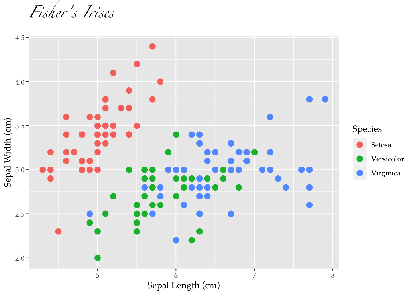
demo_plt <- ggplot(iris, aes(Sepal.Length, Sepal.Width, color=Species)) + 
  geom_point(size=3) +
  scale_color_discrete(labels=c("Setosa", "Versicolor", "Virginica")) + 
  labs(x="Sepal Length (cm)", y="Sepal Width (cm)", title="Fisher's Irises") 
demo_plt

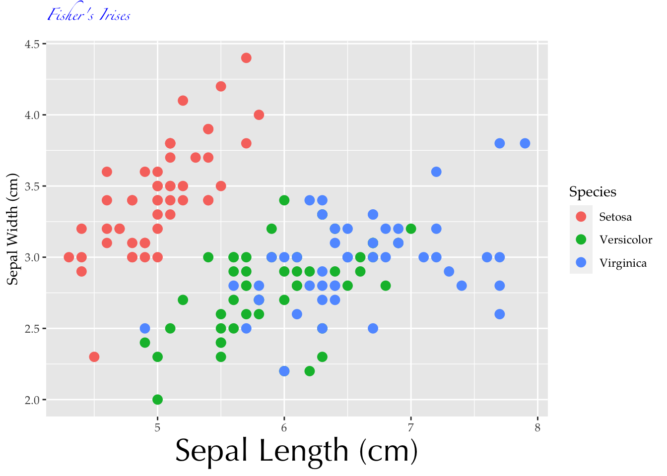
In ggplot, the theme() function lets us control the appearance of various aspects of the plot. There are many, many properties we can tweak; we will begin by setting the global text property for all text on the entire plot.

Let’s try changing that font a bit:

demo_plt + theme(text=element_text(family="Optima"))

demo_plt + theme(text=element_text(family="Palatino"))

demo_plt + theme(text=element_text(family="Zapfino"))

Note that the specific name that you must use to refer to the font is not exactly obvious. It is not the font name, but rather the font’s “family name”. Because of some under-the-hood details about the way that fonts work, this is a bit different from what you might see in e.g. a font selection menu in Word. You can see a list of all the fonts that R knows about by using the fonttable() command:

fonttable() %>% glimpse()

Rows: 149
Columns: 10
$ package    <lgl> NA, NA, NA, NA, NA, NA, NA, NA, NA, NA, NA, NA, NA, NA, NA,…
$ afmfile    <chr> "Keyboard.afm.gz", "SFNSDisplay.afm.gz", "SFNSText.afm.gz",…
$ fontfile   <chr> "/System/Library/Fonts/Keyboard.ttf", "/System/Library/Font…
$ FullName   <chr> ".Keyboard", "System Font", "System Font", "System Font Ita…
$ FamilyName <chr> ".Keyboard", "System Font", "System Font", "System Font", "…
$ FontName   <chr> "-Keyboard", "-SFNSDisplay", "-SFNSText", "-SFNSText-Italic…
$ Bold       <lgl> FALSE, FALSE, FALSE, FALSE, FALSE, FALSE, FALSE, FALSE, FAL…
$ Italic     <lgl> FALSE, FALSE, FALSE, TRUE, FALSE, FALSE, FALSE, FALSE, FALS…
$ Symbol     <lgl> FALSE, FALSE, FALSE, FALSE, FALSE, FALSE, FALSE, FALSE, FAL…
$ afmsymfile <lgl> NA, NA, NA, NA, NA, NA, NA, NA, NA, NA, NA, NA, NA, NA, NA,…

fonttable() %>% head()

package	afmfile	fontfile	FullName	FamilyName	FontName	Bold	Italic	Symbol	afmsymfile
	Keyboard.afm.gz	/System/Library/Fonts/Keyboard.ttf	.Keyboard	.Keyboard	-Keyboard	FALSE	FALSE	FALSE
	SFNSDisplay.afm.gz	/System/Library/Fonts/SFNSDisplay.ttf	System Font	System Font	-SFNSDisplay	FALSE	FALSE	FALSE
	SFNSText.afm.gz	/System/Library/Fonts/SFNSText.ttf	System Font	System Font	-SFNSText	FALSE	FALSE	FALSE
	SFNSTextItalic.afm.gz	/System/Library/Fonts/SFNSTextItalic.ttf	System Font Italic	System Font	-SFNSText-Italic	FALSE	TRUE	FALSE
	Andale Mono.afm.gz	/Library/Fonts/Andale Mono.ttf	Andale Mono	Andale Mono	AndaleMono	FALSE	FALSE	FALSE
	Apple Braille.afm.gz	/System/Library/Fonts/Apple Braille.ttf	Apple Braille	Apple Braille	AppleBraille	FALSE	FALSE	FALSE

fonttable() %>% select(FullName, FamilyName, FontName) %>% head(20)

FullName	FamilyName	FontName
.Keyboard	.Keyboard	-Keyboard
System Font	System Font	-SFNSDisplay
System Font	System Font	-SFNSText
System Font Italic	System Font	-SFNSText-Italic
Andale Mono	Andale Mono	AndaleMono
Apple Braille	Apple Braille	AppleBraille
Apple Braille Outline 6 Dot	Apple Braille	AppleBraille-Outline6Dot
Apple Braille Outline 8 Dot	Apple Braille	AppleBraille-Outline8Dot
Apple Braille Pinpoint 6 Dot	Apple Braille	AppleBraille-Pinpoint6Dot
Apple Braille Pinpoint 8 Dot	Apple Braille	AppleBraille-Pinpoint8Dot
AppleMyungjo Regular	AppleMyungjo	AppleMyungjo
Arial Black	Arial Black	Arial-Black
Arial Bold Italic	Arial	Arial-BoldItalicMT
Arial Bold	Arial	Arial-BoldMT
Arial Italic	Arial	Arial-ItalicMT
Arial	Arial	ArialMT
Arial Narrow	Arial Narrow	ArialNarrow
Arial Narrow Bold	Arial Narrow	ArialNarrow-Bold
Arial Narrow Bold Italic	Arial Narrow	ArialNarrow-BoldItalic
Arial Narrow Italic	Arial Narrow	ArialNarrow-Italic

fonttable() %>% select(FamilyName) %>% distinct()

FamilyName
.Keyboard
System Font
Andale Mono
Apple Braille
AppleMyungjo
Arial Black
Arial
Arial Narrow
Arial Rounded MT Bold
Arial Unicode MS
Bitter
Bodoni Ornaments
Bodoni 72 Smallcaps
Brush Script MT
Calibri
Calibri Light
Comic Sans MS
Consolas
Courier New
DIN Alternate
DIN Condensed
Fira Sans Black
Fira Sans
Fira Sans ExtraBold
Fira Sans ExtraLight
Fira Sans Light
Fira Sans Medium
Fira Sans SemiBold
Fira Sans Thin
Fondamento
Georgia
Gorni
Impact
Karla
Khmer Sangam MN
Lao Sangam MN
Lato Black
Lato
Lato Hairline
Lato Light
Luminari
Microsoft Sans Serif
Noto Sans
Noto Serif
Open Sans
Open Sans Extrabold
Open Sans Light
Open Sans Semibold
SILDoulos IPA93
SILManuscript IPA93
SILSophia IPA93
Tahoma
Tangerine
Times New Roman
Trattatello
Trebuchet MS
Verdana
Webdings
WeePeople
Wingdings
Wingdings 2
Wingdings 3
.SF NS Rounded
Harding Text Web Bold
Harding Text Web Regular

Long story short, you’ll want to use the value in FamilyName to refer to your font of interest.

What if we wanted to have a different font for the title? The plot.title property is where we would want to look:

demo_plt + theme(
  text=element_text(family="Palatino"),
  plot.title=element_text(family="Zapfino")
  )

We can follow this pattern to change anything we like about the text in different parts of the plot:

demo_plt + theme(
  text=element_text(family="Palatino"),
  plot.title=element_text(family="Zapfino", size=8, color="blue"),
  axis.title.x = element_text(family="Optima", size=24)
  )

7.2 Installing new fonts

This part is a bit beyond the scope of this class, but the upshot is that after you install new fonts in your computer, you should tell extrafont about it using the font_import() command.

7.2.1 Caveats

extrafont only knows about TrueType fonts (ones whose file ends in .ttf). If you have an OpenType font you want to use with R, your best bet probably involves the showtext package.